Nourden Mohamed Abdelsadeg¹

Department of Chemical and Petroleum Engineering, Elmergib University, Libya

Email: nmabdelsadeg@elmergib.edu.ly

HNSJ, 2023, 4(2); https://doi.org/10.53796/hnsj4220

Download

Published at 01/02/2023 Accepted at 05/01/2023

Abstract

The most commonly used method to predict the initial stabilized deliverability potential of a gas well is the modified isochronal test that includes an extended flow period to pressure stabilization. Some reservoirs do not period to pressure stabilization. Some reservoirs do not attain stabilization even after 100 or more hours of now and consequently a reliable, extended flow period on such reservoirs can be unreasonably expensive and wasteful.

Predicting and assuring well deliverability often are important concerns when developing gas condensate reservoirs. Also, it is bind with the long-term contracts where it is needed to assure gas well deliverability and sustainability for long period.

This paper takes well BB5 gas well located in Faregh field that operated by WAHA oil company as case of study to analysis isochronal test using different methods to estimate the maximum gas rate and construct IPR curve, 92.56 MMSCF/D was the maximum gas rate using empirical method, 89.06 MMSCF/D was the maximum gas rate using modified method, 84.58 MMSCF/D was the maximum gas rate using Extract method. And by three different methods shows the difference slightly small between methods and the average maximum gas rate is 89.06 MMSCF/D.

In PROSPER model the maximum gas rate was 91.483 MMSCF/D and this value was close to the value from the analysis of EXCEL SHEET. Finally, the main target of this paper is to construct the IPR of this gas well using different methods and the IPR’s with different methods using EXCEL sheet and PROSPER to be used to predicted the performance of this gas well.

Key Words: Isochronal Test, PROSPER software, Inflow Performance Relationship, Gas Rate.

عنوان البحث

إستخدام بيانات الاختبار المتزامن لتحديد سعة التدفق لبئر غاز باستخدام طرق مختلفة: دراسة حالة لحقل الفارغ، ليبيا.

نور الدين محمد عبد الصادق¹

¹ قسم الهندسة الكيميائية والبترولية ، جامعة المرقب ، ليبيا

بريد إلكتروني: nmabdelsadeg@elmergib.edu.ly

HNSJ, 2023, 4(2); https://doi.org/10.53796/hnsj4220

تاريخ النشر: 01/02/2023م تاريخ القبول: 05/01/2023م

المستخلص

من الطرق الأكثر شيوعًا للتنبؤ بإمكانية التسليم المبدئي المستقرة لبئر غاز هي الاختبار المتساوي الزمني المعدل ، والذي يتضمن فترة تدفق ممتدة لاستقرار الضغط. بعض الخزانات لا تستغرق فترة للضغط لكي يستقر. وبعض الخزانات لا تحقق الاستقرار حتى بعد 100 ساعة أو أكثر من الآن ، وبالتالي فإن فترة التدفق الموثوق بها والممتدة على هذه الخزانات يمكن أن تكون باهظة الثمن ومهدرة بشكل غير معقول.غالبًا ما يكون التنبؤ والتأكد من قابلية تسليم البئر من الاهتمامات المهمة عند تطوير خزانات مكثفات الغاز. كما أنه ملزم بالعقود طويلة الأجل حيث يكون ضروريًا لضمان إمكانية تسليم بئر الغاز واستدامته لفترة طويلة.

يتناول هذا البحث بئر غاز (BB5) الموجود في حقل الفارغ الذي تديره شركة النفط الواحه كحالة دراسة لتحليل اختبار متساوي الزمن باستخدام طرق مختلفة لتقدير الحد الأقصى لمعدل الغاز و إنشاء منحنى IPR الحد الاقصى للغاز كان MMSCF/D 92.56 باستخدام الطريقة التجريبية وكان MMSCF/ D 89.06 هو الحد الاقصى لمعدل الغاز باستخدام الطريقة المعدلة وكان MMSCF/D 84.58 هو اقصى معدل للغاز باستخدام طريقة الاستخراج. وبواسطة الطرق الثلاث المختلفة يظهر الاختلاف بسيط بين الطرق ومتوسط الحد الاقصى لمعدل الغاز هو MMSCF/D89.06 وهذه القيمة قريبه من المتحصل عليها باستخدام لاكسل.

الهدف الرئيسي من هذه الورقة هو إنشاء حقوق الملكية الفكرية لبئر الغاز وهذا باستخدام طرق مختلفة و IPR بطرق مختلفة باستخدام ورقة EXCEL و PROSPER لاستخدامها للتنبؤ بأداء بئر الغاز هذا.

1. Introduction

General Background

In the world of reservoir engineering, well testing is one of the most applicable tools for estimating reservoir parameters and evaluating of well conditions. Most of the proposed approaches for well testing are based on diffusivity equation in which several assumptions simplify the problem. Single phase flow of liquid and uniform thickness is some of these assumptions, whereas the behavior of reservoir changes to multi-phase after a period of production. Dissolved gas and gas condensate are examples of these types of reservoirs. In recent years, several researches have focused on studying the gas condensate reservoirs because of their importance [1] [2].

For gas-condensate reservoirs, generally, the hydrocarbons are completely in gas phase at initial conditions while the condensate starts to evolve during an isothermal process of pressure drop. The condensate will accumulate to a maximum value (maximum liquid drops out percentage measured during CVD experiment) then starts to vaporize again to gas phase and this reverse behavior in gas condensate reservoir phenomenon is referring to as “retrograde condensation”. However, the generation of liquids will stop if the pressure reduction continues [2] [3].

The condensates are a mixture of liquid and gas fluids whereas the liquid part is more valuable; therefore, it is more desirable for Petroleum Companies to recover as much as condensate at the surface. In the case of substantial condensate drop out in the reservoir, the gas relative permeability would be impaired, and as a result, production of gas with lower condensate content will not be feasible any more [1].

This study was conducted on a gas condensate development well of Farag field, operated by WAHA oil company.

A modified isochronal test is a useful tool in evaluating a well productivity and formation parameters of a gas well [1] [3]. Pressure test analysis was performed to investigate the success of the well completion and well performance during production with different scenarios. Inflow performance curves, and pressure and production forecasts were also performed using transient pressure analysis as well as using derivability test analysis methods [4].

Objectives of Paper

The main objectives of this paper summarized as following:

1. Collecting the required real data for the study
2. Analyze the isochronal test for gas condensate well, derivability test by using different techniques (empirical, modified and exact methods) to develop general Inflow Performance Relationship (IPR) curve.
3. Well modelling using PROSPER software to analysis the isochronal test for gas condensate well to develop general Inflow Performance Relationship (IPR) curve.
4. Finally, comparison the results of test that developed form Excel and results from well Modelling PROSPER software.

Case Study: Faragh Oil Field

Field General Background

The Faregh Field is located in the southeastern portion of the Sirt Basin (Figure 2.1). Drilling in Faregh commenced in 1962 and hydrocarbons were discovered in 1963 in BB-1, which was tested gas when completed. To date a total of 62 wells have been drilled consisting of 41 Exploration wells and 21 Development wells. A total of nine (9) reservoirs pools have been discovered (5I, EE, BB, 5A, 3U, 4D, 4T, 5H, and 6B). A total of 38 wells are capable of oil and/or gas production from these pools. Nineteen wells have been plugged and abandoned [5].

Figure 2.1 shows a structure map in the field. Two pools, 5I and EE, contain large oil legs and gas cap reserves. Two pools, BB and 5A have thin oil legs with large gas caps. Five other pools, 3U, 4D, 4T, 5H and 6B are much smaller. The oil and gas bearing reservoirs produce from either the Amrha and Faregh sands of the Sarir formation with minor reserves in the Etla from well BB2A.

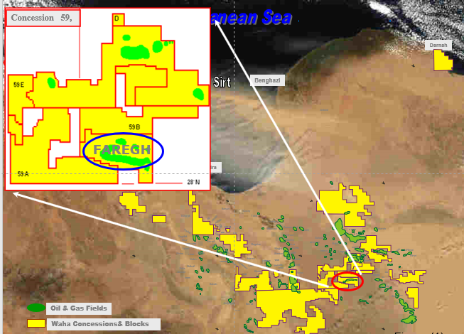
Figure 2.1: Field location Background

The development plan for Phase 1 is to produce oil from 23 vertical wells with oil rim perforations selected from the 50 wells drilled to delineate the various reservoirs. The intention was to access the oil-rim and maximize oil recovery prior to the Phase 2 gas cap development. Commissioning of Phase I facilities commenced on April 19, 2003 and is still ongoing.Phase 2 is planned as a gas cap development with expected off-take of 180 MMSCFD and 15 MBPD of condensate. Commissioning of Phase II facilities commenced on November 19, 2010.

Reservoir Description

The Faregh field has two high quality sandstone reservoir intervals, namely Faregh and Amarha. Both of these reservoir units are dominated by relatively clean, mature, quartz sandstones mostly deposited in a series of stacked braided channels. The younger Faregh Sandstone is interpreted to have been deposited within a broader group of depositional environments, with cores displaying evidence of continental braidplains, transitioning to deltaic and estuarine / lacustrine settings. The Amrha reservoir appears to be overwhelmingly dominated by stacked channels that were deposited in a braided plain setting based on core description. The Amrha Sandstone is underlain by a variable succession of sandstones, siltstones and claystones, which constitute the lowermost unit of the Nubian section called El Abd. The El Abd sedimentology is characterized by a broad variety of grain sizes, sediment maturities, and sedimentary structures. The El Abd unit is underlain by igneous, metamorphic, and sedimentary rocks, which ultimately rests on Precambrian crystalline basement. The El Tami Shale separates the Amrha Sandstone from the Faregh Sandstone and is likely equivalent to the Middle Nubian Shale (also called Variegated Shale), recognized elsewhere in the region. Locally within the Faregh Field, however, the El Tami section includes volcanic beds. The unit is largely composed of silts and very fine sandstones, with locally thick shale beds.

The log-derived porosity typically averages between 9% and 12% per analyzed interval and is largely primary in nature. Core derived permeability ranges between 1.5 to 180 mD for the Amrha. The oil reservoir in the Nubian section is very similar throughout the area, being typically 39-42° API with a high wax content. The fields have a common structural history, trapping mechanism and reservoir properties. The reservoir stratigraphy classification for the Faregh Field is shown in Figure (2.2) [5].

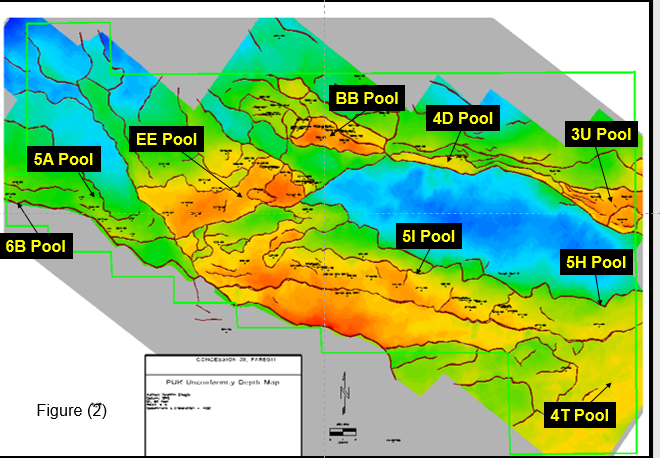
Figure 2.2: Reservoirs Background

Production Performance History

The oil production (Phase I) commenced in April 2003. The average daily oil production rate during 2010 was 15,328 BOPD (17,778) during December 2010. The average daily gas production rate during 2010 was 48.6 MMSCFPD (52.5) during December 2010. The GOR trend from most of the wells’ production and test data indicated that the wells are producing at high GOR. The increase in the GOR in excess of the solution GOR could be attributed to either coning from the gas cap or gas is being produced directly from the gas cap through the annular behind the casing due to boor cement job. The oil production rate is limited by shutting-in high GOR wells in order to reduce gas flaring. The production capacity of the reservoir is estimated to be about 25,000 BOPD based on the December 2010 production rates for producing wells and the latest previous production rates for shut-in wells [5]. The cumulative oil and gas production as of 2010 are 33.15 MMSTB and 121.19 BSCF respectively.

The single pool and total field Production history. The data is plotted as calendar day rates which incorporate any shut-in periods within each month [5].

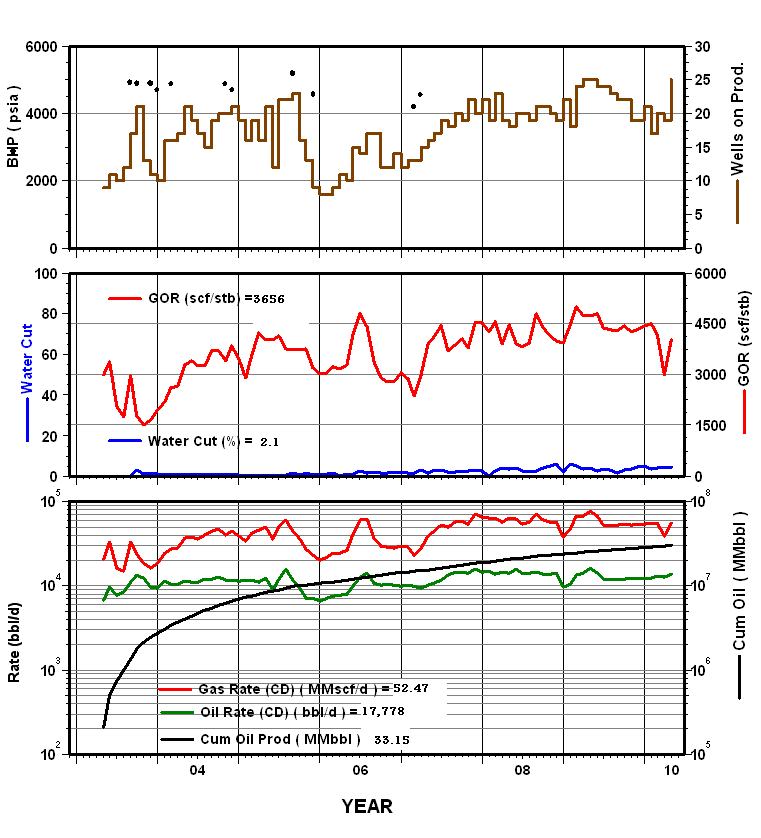
Figure 2.3: Production Performance

Original Oil and Gas in Place

The currently Booked Original Oil-in-Place (OOIP) and Recoverable Oil Reserves are 845.4 MMSTB and 127.3 MMSTB, respectively while the currently Booked Original Gas in-Place (OGIP) and Recoverable Gas (Associated & Non-Associated) reserves are 3620.79 BSCF and 2215.71BSCF, respectively. These estimates were based on the results of the 1987 reservoir study by Scientific Software Corporation (SSI) [5][6].

The recently completed reservoir study has indicated that the estimated original oil and gas in place are 1809 MMSTB and 5893 BSCF respectively. The total oil and gas recovery over 50 years (Case J2) are 370 MMSTB and 3.7 TSCF respectively.

Horizontal wells in Faregh field drilled in the oil rim; to improve oil recovery by contacting and capturing more oil and reducing gas coning relative to a vertical completion. The lower gas-oil ratio will make a significant contribution to increasing oil reserve recovery and to produce the reserves in a timely manner [5].

As a continuation of Faregh Development Drilling Plan; two horizontal oil wells were drilled in the “5I” pool. Well, 5I17 was spudded in December 2009; while 5I18H was spudded at the end of October 2009. The drilling operations for both wells were completed in February 2011. exhibits the open log interpretation for 5I17H and 5I18H. Logs data indicate both wells are likely to produce around 2000 BOPD. In addition, two infill oil wells will be drilled according to “2011 Development Drilling Plan”. Both wells will be drilled horizontally in “BB Pool” to expedite oil recovery [5][6][7].

Results and Discussion

Analysis and Results

In this paper actual field data for Faregh field was collected as pdf file contains the results of isochronal test that run in 24/12/2008 as test with different chock size and measured wellhead pressure, wellhead temperature, casing pressure, gas rate, oil rate, water rate and total gas oil ratio as shown in Figure (3.1).

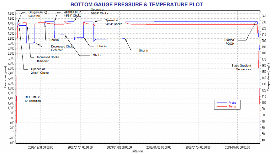
Figure ‎3: bottom gauge pressure and temperature (isochronal test)

As shown in table (3.1) the test start with 24/64 chock size then shut in period for 6 hrs, then 48/64 chock size then shut in period for 6 hrs, then 56/64 chock size then shut in period for 6 hrs also, finally 64/64 chock size and produce for 16 hrs then shut in for 72 hrs for buildup test.

Table 3.1: Full Set of Isochronal Test Data

Data
Chock	Date	Duration Flowing Time	Gas Flow Rate	Oil Flow Rate	Water Flow Rate	Flowing Bottom Hole Pressure	Duration for Build Up	Bottom Hole Pressure
/		hr	MMScf/Day	bbl/Day	bbl/Day	Psia	hr	Psia
24	30-Dec-08	4	8.096	527	21.9	4312	6	4467
48	31-Dec-08	4	23.013	1383	104.1	3930	6	4465
56	31-Dec-08	4	26.166	1500	112.9	3820	6	4466
64	1-Jan-09	16	29.623	1548	116	3760	72	4465

Deliverability Test Analysis (Excel Sheet)

It executed deliverability test analysis for a well by using Excel sheet to construct IPR curve with three different methods (empirical, modified and extract) and the analysis below showed the results for these methods as following:

• • 1. Empirical method

The analysis starts by calculations of n and C coefficient figure (3.2) shown the calculation of slop to determine (n) and the value of n= 0.8802 then calculate C=3.473e-5.

Table 3.2: Full Set of Isochronal Test Data

Chock	Gas Flow Rate	Oil Flow Rate	Water Flow Rate	Corrected Gas Flow Rate	(Pe^2-Pwf^2)	Inflow Coefficient
/	MMScf/Day	bbl/Day	bbl/Day	MMScf/Day	Psia	MMScf/Day/Psia^2
24	8.096	527	21.9	8.720	1360745	3.4784E-05
48	23.013	1383	104.1	24.995	4491325	3.48524E-05
56	26.166	1500	112.9	28.316	5352756	3.38322E-05
64	29.623	1548	116	31.838	5798625	3.54534E-05

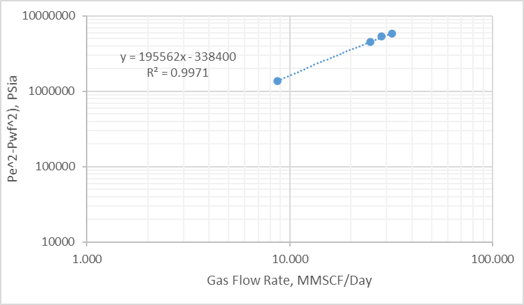
Figure 3.2: Empirical Methods Analysis

Figure (3.3) and Table (3.3) shows the results of calculation of IPR of well using the isochronal test

Table 3.2: IPR Calculations using (Empirical Method)

IPR Calculation (Empirical Method)
		Flowing pressure	Flow Rate
Psia	MMSCF
4467	0.00
4300	9.29
4100	18.20
4000	22.27
3900	26.14
3500	40.05
3000	54.60
2000	76.01
1000	88.46
500	91.54
15	92.56

In this method the maximum gas rate from of the well was 92.56 MMSCF/D as shown clearly in figure (3.3).

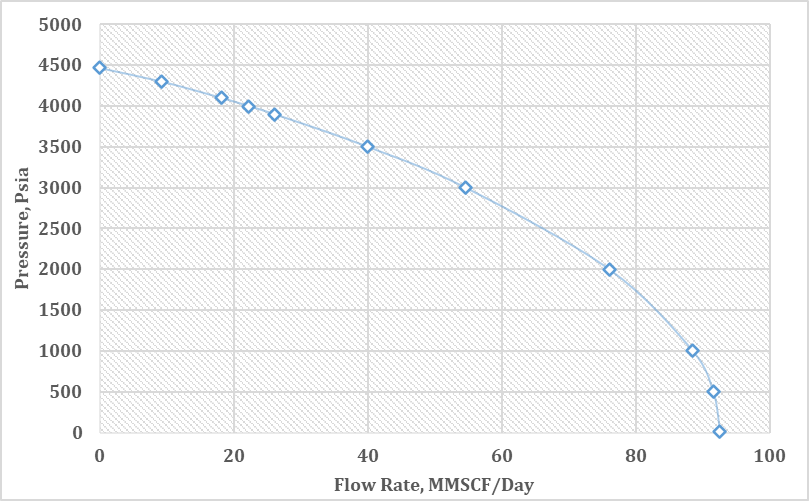
Figure 3.3: IPR Calculation using Empirical Methods Analysis

• • 1. Modified method

The analysis starts by calculations of a and b coefficient figure (3.4) shown the calculation of slop to determine (a) and the value of a= 0.1063 then calculate b=0.00132

Table 3.4: Isochronal Test Data (Modified)

Chock	Gas Flow Rate	Oil Flow Rate	Water Flow Rate	Corrected Gas Flow Rate	(Pe^2-Pwf^2)/qg
/	MMScf/Day	bbl/Day	bbl/Day	MMScf/Day	Psia
24	8.096	527	21.9	8.720	0.1560
48	23.013	1383	104.1	24.995	0.1797
56	26.166	1500	112.9	28.316	0.1890
64	29.623	1548	116	31.838	0.1821

Table 3.5: IPR Calculations using (Modified Method)

IPR Calculation (Modified Method)
		Flowing pressure	Flow Rate
Psia	MMSCF
4467	0.00
4300	11.99
4100	23.00
4000	27.67
3900	31.94
3500	46.07
3000	59.30
2000	76.77
1000	86.10
500	88.32
15	89.06

Figure (3.4) and Table (4.4) shows the results of calculation of IPR of well using the isochronal test with modified method of calculation.

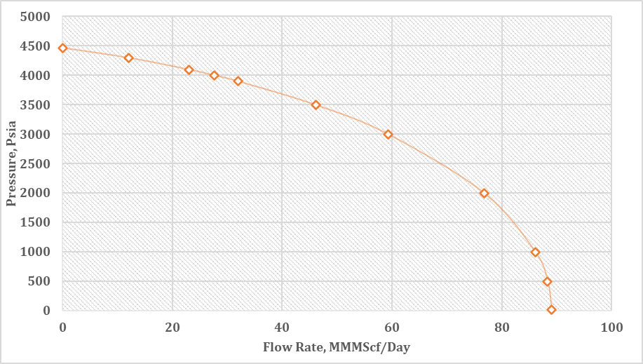
Figure 3.4: IPR Calculation using Modified Methods Analysis

In this method the maximum gas rate from the well was 89.06 MMSCF/D as shown clearly in figure (3.4).

• • 1. Extract method

The analysis starts by calculations of a and b coefficient figure (3.5) shown the calculation of slop to determine (a) and the value of a= 7*10⁶ then calculate b=7*10⁷

Table 3.6: Isochronal Test Data (Modified)

Chock	Gas Flow Rate	Oil Flow Rate	Water Flow Rate	Corrected Gas Flow Rate	(Pe^2-Pwf^2)/qg
/	MMScf/Day	bbl/Day	bbl/Day	MMScf/Day	Psia
24	8.096	527	21.9	8.720	4055119872
48	23.013	1383	104.1	24.995	5320538072
56	26.166	1500	112.9	28.316	5761598687
64	29.623	1548	116	31.838	5634703804

Table 3.7: IPR Calculations using (Extract Method)

IPR Calculation (Extract Method)
		Flowing pressure	Flow Rate
Psia	MMSCF
4467	0.00
4392	4.45
4323	8.90
4241	13.35
4148	17.81
4042	22.26
3925	26.71
3795	31.16
3653	35.61
3498	40.06
3329	44.51
3147	48.97
2949	53.42
2733	57.87
2496	62.32
2234	66.77
1935	71.22
1582	75.68
1123	80.13
15	84.58

Figure (3.5) and Table (3.7) shows the results of calculation of IPR of well using the isochronal test with Extract method of calculation.

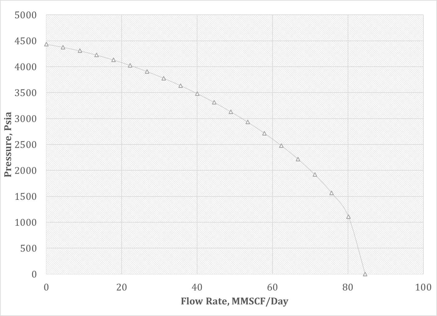
Figure 3.5: IPR Calculation using Extract Methods Analysis

In this method the maximum gas rate from the well was 84.58 MMSCF/D as shown clearly in figure (3.5).

Figure (3.6) shows the IPR curve with the three different methods and shows the difference slightly small between methods and the average maximum gas rate is 89.06 MMSCF/D.

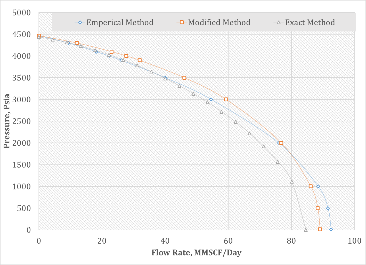
Figure 3.6: IPR Calculation using ALL Methods of Analysis

• • 1. Deliverability Test Analysis (Excel Sheet)

Prosper, Petroleum Experts Limited’s advanced production and systems performance analysis software. Prosper can assist the production or reservoir engineer to predict tubing and pipeline hydraulics and temperatures with accuracy and speed. Prosper powerful sensitivity calculation features enable existing designs to be optimized and the effects of future changes in system parameters to be assessed [8][9].

This paper uses Prosper software to construct inflow performance relationship by using available methods, the Prosper software includes the main steps in order to construct IPR curve these are:

1. Options Summary
2. PVT Data
3. IPR Data

Input Data

• Option Summary

To begin setting up the system options, make the following selections:

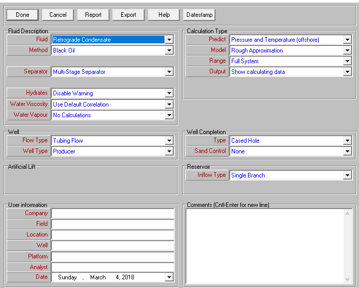
Figure 3.7: Option Summary for Well BB5

This completes the main system setup and re-initializes the program. If the status screen is being displayed, the main system areas (‘PVT DATA’, ‘EQUIPMENT DATA’ and ‘IPR Data’) can be now easily accessed.

• PVT Data

The purpose of this section is to demonstrate how to enter the PVT model and to match the PVT correlations to real PVT data.

The steps we will follow are the following:

1. Enter PVT Black Oil model.

A09)

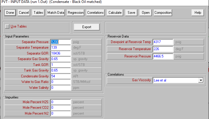
Figure3.8: Black Oil Model for well BB5

Enter PVT match data.

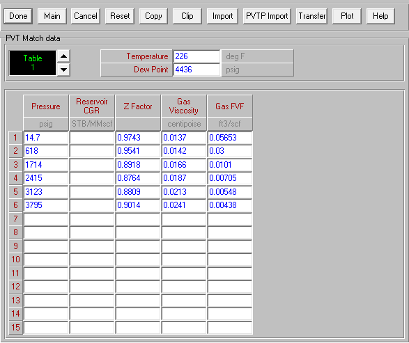
Figure 3.10: PVT Match Data for well BB5

1. Match the PVT Black Oil correlations to the PVT match data entered and choose the best correlation.

To match the correlations to the laboratory measured data, from the main PVT input data screen select Regression:

(A09)

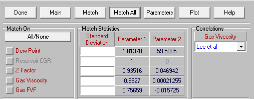
Figure 3.11: Regression Option

Then select match all to run the regression calculation. At this point the program performs a non-linear regression to adjust the correlations to best fit the laboratory data by applying a multiplier (Parameter 1) and a shift (Parameter 2) to each the correlations.

To be noticed also the flashing green message PVT is Matched showing that the PVT model has been matched. Figure (3.11) illustrates gas formation volume factor versus pressure, the gas deviation factor and gas viscosity versus pressure plotted in (Figure 3.12 & 3.13) respectively.

(A09)

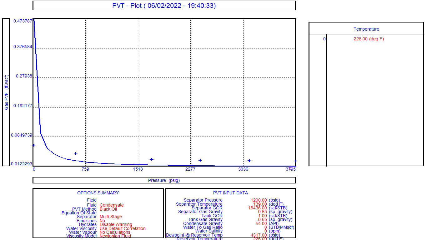
Figure 3.11: Gas FVF versus pressure for well BB5

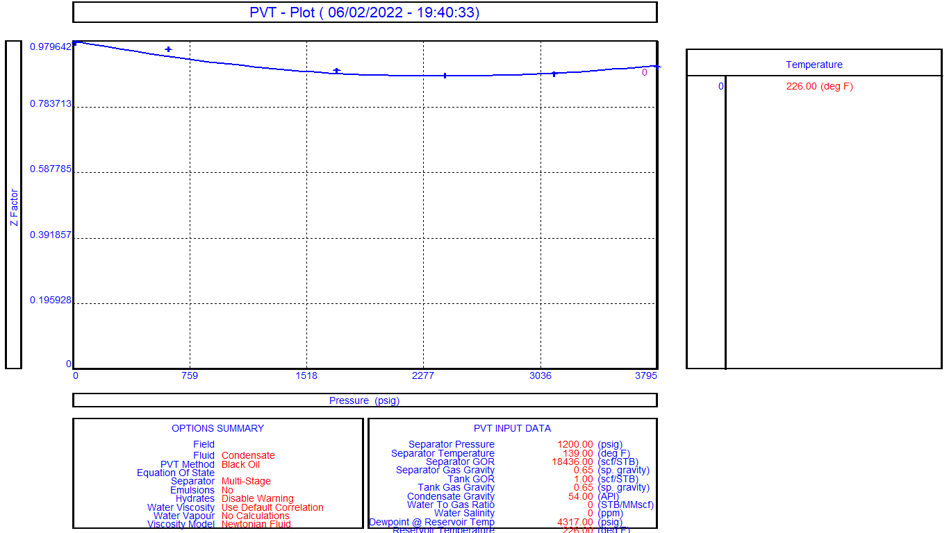
Figure 3.12: Gas deviation factor versus pressure for well BB5

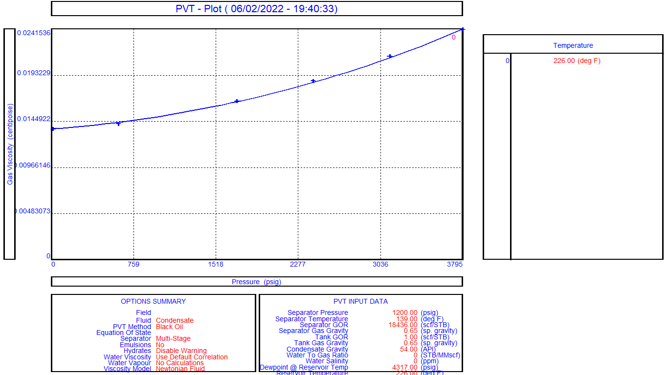
Figure 3.13: Gas viscosity versus pressure for well BB5

The next task is to enter the Inflow Performance model. In this study was selected MULTIRATE C and n to construct IPR curve.

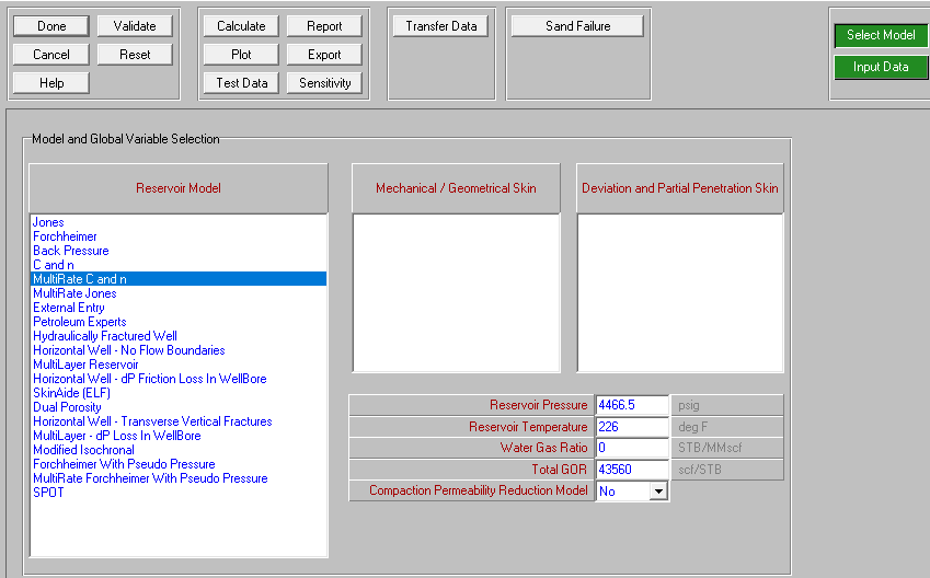
Figure 3.14: IPR Methods Interface

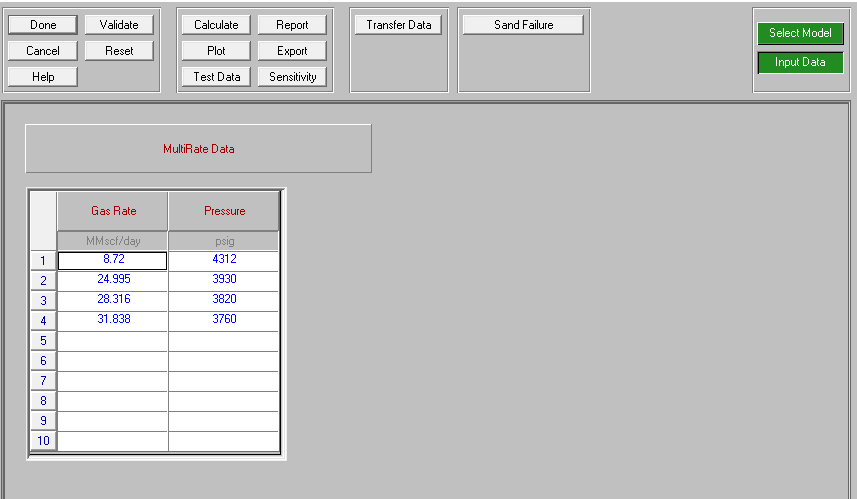
Figure 3.15: Input Data for Multi rate Method

The input data for this method illustrated in (Figure 3.15).

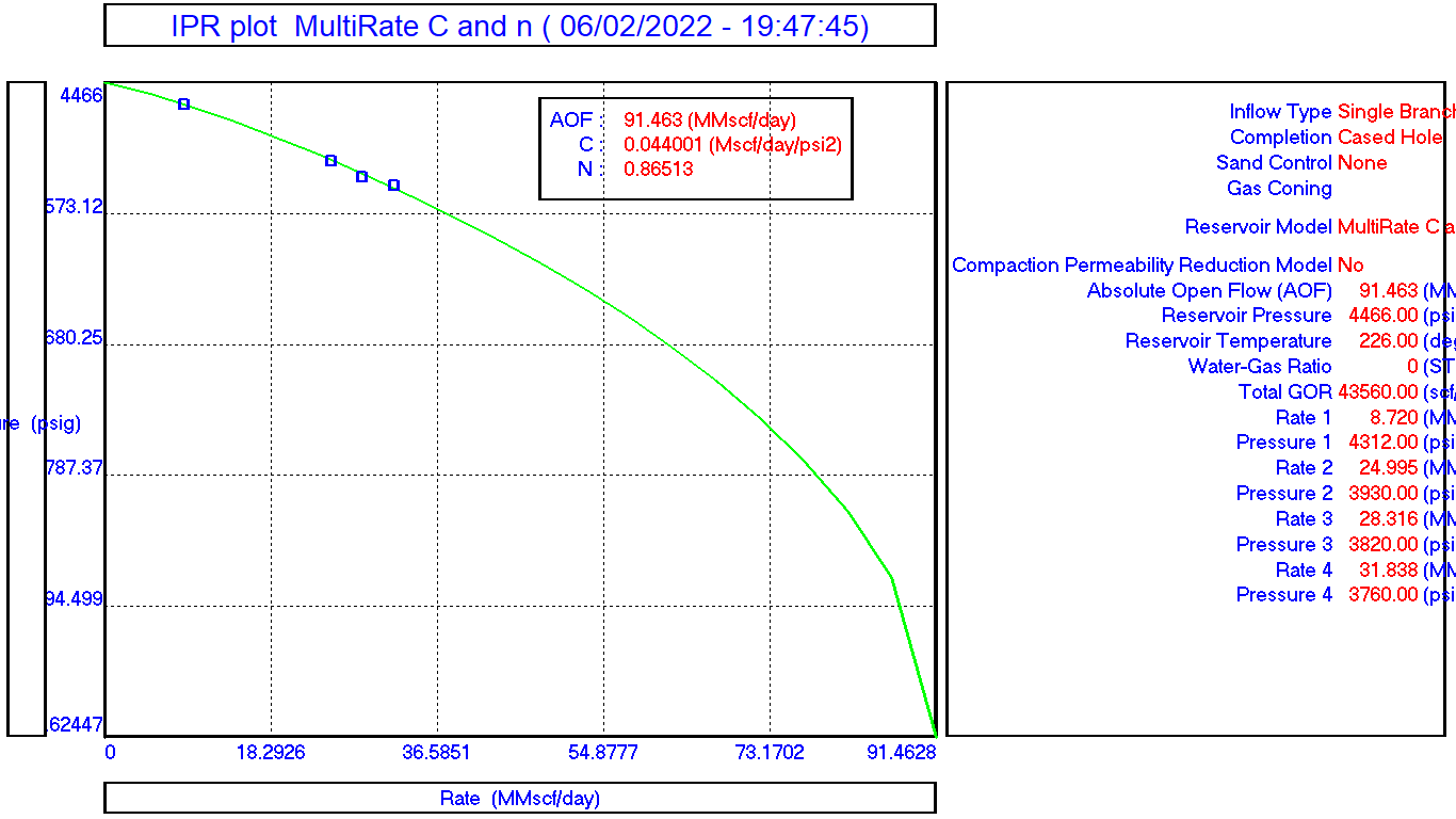
Figure 3.16: IPR Curve using MULTI RATE method for well BB5

In this method the maximum gas rate from the well was 91.483 MMSCF/D as shown clearly in figure (3.16).

Finally, the main target of this study is to construct the IPR of this gas well using different methods and the Figure (3.17) shows the IPR’s with different methods using EXCEL sheet and PROSPER to be used to predicted the performance of this gas well.

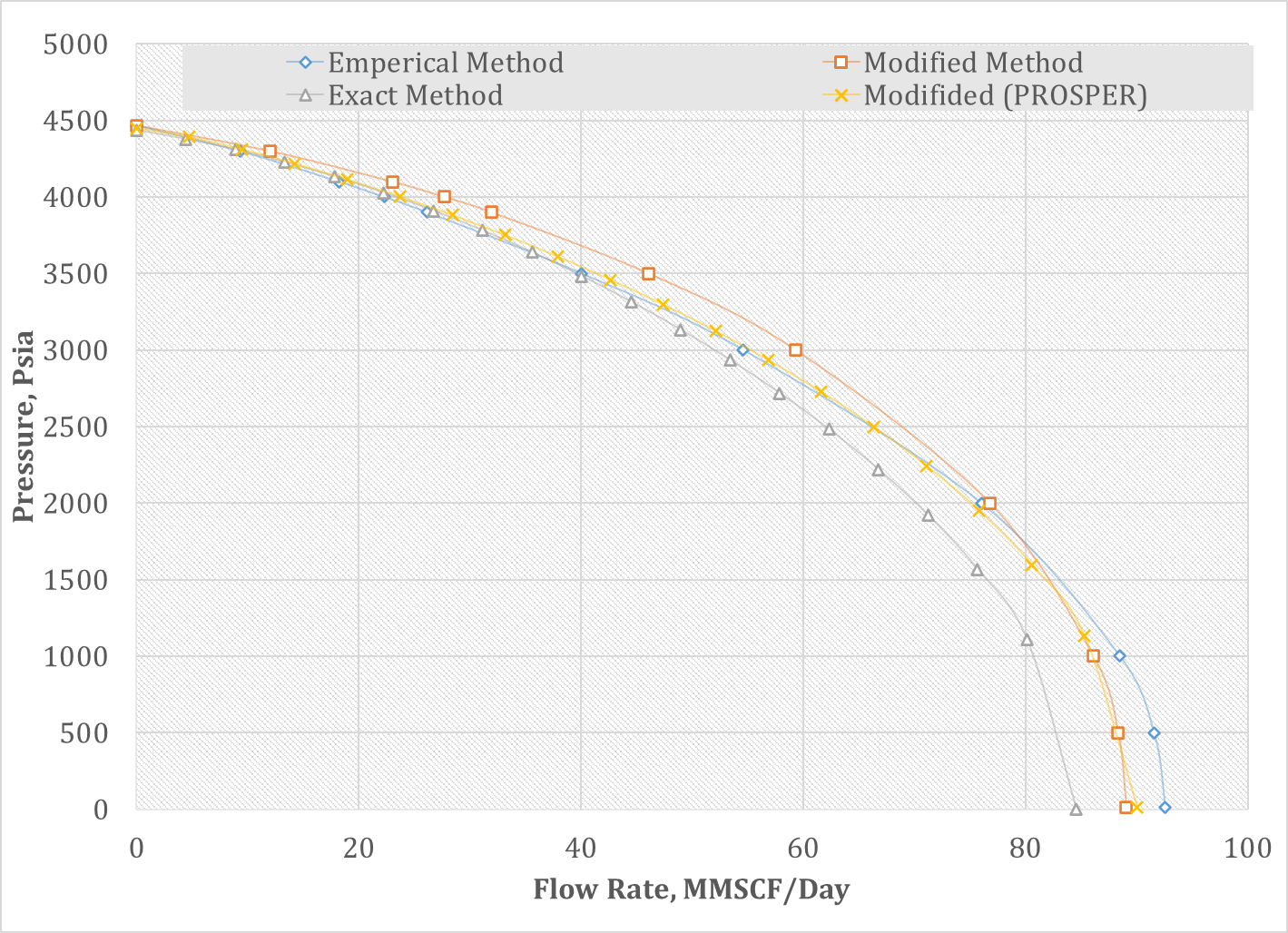
Figure 3.17: IPR Curve using Different methods for well B

Conclusions and Recommendations

Conclusions

The main Conclusions of this project can be summarized as follows:

1. In this study take well BB5 gas well located in Faregh field that operated by WAHA Oil Company as case of study to analysis isochronal test using different methods to estimate PI.
2. The test starts with 24/64 chock size then shut in period for 6 hrs, then 48/64 chock size then shut in period for 6 hrs, then 56/64 chock size then shut in period for 6 hrs also, finally 64/64 chock size and produce for 16 hrs then shut in for 72 hrs for buildup test with maximum gas rate 29.623 MMScf/Day.
3. 92.56 MMSCF/D was the maximum gas rate using empirical method.
4. 89.06 MMSCF/D was the maximum gas rate using modified method
5. 84.58 MMSCF/D was the maximum gas rate using Extract method.
6. Using three different methods shows the difference slightly small between methods and the average maximum gas rate is 89.06 MMSCF/D.
7. In PROSPER model the maximum gas rate was 91.483 MMSCF/D and this value close to the value from the analysis of EXCEL SHEET.
8. The overall objective of this paper was achieved which is to construct the IPR of this gas well using different methods and the IPR’s with different methods using EXCEL sheet and PROSPER to be used to predicted the performance of this gas well.

Recommendations

Complete the analysis of BUILDUP test to estimation of reservoir parameters and skin factor to evaluate the well future performance.

References

1. Tarek Ahmad – Reservoir Engineering Handbook third Edition.
2. Urayet A.A: ”Oil Property Evaluation” University of Tripoli, Tripoli, 1998
3. J. J. Arps, “Analysis of Decline Curves,” Trans., AIME (1944).
4. Du Y, Guan L and Li D. Deliverability of wells in the gas condensate reservoir. 11th ADIPEC Abu Dhabi International Petroleum Exhibition & Conference, 10-13 Octobers 2004, Abu Dhabi (SPE 88796)
5. Waha Oil Company, Planning Engineering Department (2022)
6. Barry K. Vansandt et al. “Gaudiness for Application Definitions for Oil and Gas Reserves” Dec. 1988.
7. J U. A. A., Advanced Gas Reservoir Engineering Tripoli. 2014
8. Fussell, D.D.: “Single-Well Performance Predictions for Gas Condensate Reservoirs,” JPT (July 1973)
9. Schlumberger, Fundamental of Formation Testing, )2002(.
10. Ayy alasomayajula P, Silpngarmlers N and Kamath J. Well deliverability predictions for a low-permeability gas/condensate reservoir. SPE Annual Technical Conference and Exhibition,) October 2005(, Dallas, Texas (SPE 95529)
11. Qin B, Li X F and Cheng S Q. Gas condensate two phase flow performance in porous media considering capillary number and nonDarcy effects. Petroleum Science. 2004.