Eslam Ali Eldharif1 Taha Manour Fanoush2
Computer Science Department University of Benghazi, Benghazi, Libya
Email: eslam.alaraibi@uob.edu.ly
2 Computer Science Department University of Benghazi, Benghazi, Libya
Email: tfanoush@gmail.com
HNSJ, 2024, 5(2); https://doi.org/10.53796/hnsj52/17
Published at 01/02/2024 Accepted at 12/01/2024
Abstract
Abstract— In the contemporary era, the number of vehicles on the roads has been growing exponentially, which raised the need to automate the process of controlling traffic violations. In this work, we aim to develop a license plate recognition method using the Optical Character Recognition technology and Google Brain’s Tensorflow classification library to accomplish the mission of extracting and recognizing characters from license plate images. Moreover, this method can also be helpful for other character recognition applications.
Key Words: raster; pixel; gray-scaling; binarization; threshold; connected component; optical character recognition; image classification
- Introduction
According to the automotive trade journal Ward’s Auto, the total number of vehicles on the roads has crossed 1 billion vehicles during the year 2010 [1]. Therefore, new challenges have emerged for traffic police, such as red-light violations, speed limit violations and parking problems. Consequently, in order to control and overcome these challenges, the traffic police authorities should consider installing surveillance devices, such as red-light cameras or parking booth cameras at the crossroads, highways and parking lots, to keep track of vehicles on the road. However, the unique number on the vehicle license plate can be used to identify all vehicles in a certain region. Therefore, the license plate number is the primary and the most widely accepted identifier for all vehicles around the globe. However, it would require a huge labor force to check the images, note down the vehicle’s registration number and finally forward it to the competent authorities. Accordingly, we had to come up with a technique that makes the computer able to recognize the Libyan vehicle license plate number.
As indicated in Fig.1, the current Libyan license plates are of two forms, the rectangle-like form that has only one line of characters/numbers and the square-like form that has two lines of characters/numbers.

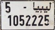
Figure 1. The two forms of the current Libyan license plate.
To identify and read this kind of license plates, several image- processing algorithms need to be implemented on the footage that was taken by the surveillance device in order to convert that image into text format before it can be used by other parts of the system. Accordingly, what we aim to develop is an Automatic License-Plate Recognition (ALPR) system that is capable of manipulating the license-plate image, and reading the characters/numbers on that image. ALPR is a combination of several techniques, such as object detection, image processing and pattern recognition. It is also known as automatic vehicle identification, car plate recognition, automatic number plate recognition, and optical character recognition (OCR) for cars [2]. OCR is the electronic conversion of handwritten, typewritten or printed text from still or motion images to machine-encoded text. Other common uses include scanning of books for electronic retrieval or scanning to edit documents electronically [3].
We believe that the development of such system can be very beneficial, and considering the conclusions and the satisfying results that were attained, we think this work represents an “added value” to the scientific researches in this field.
- Materials and Methods
This section will illustrate the concepts and techniques that were used and how are they going to help in accomplishing the mission successfully. It will also include an analysis of the problems and issues that might appear during the implementation, and a suggestion of a design for an algorithm that will definitely overcome these challenges.
- Pixels and Images
A pixel or a ‘Picture Element’ is a single squared point in an image. Moreover, images are generally displayed by dividing the screen that is displaying the image into hundreds of thousands or maybe millions of pixels, arranged in rows and columns, although the distance between these pixels is so small that they would appear connected. However, on color monitors, each pixel is actually composed of three dots: red, green and blue, as they should all assemble at the same point admirably [4]. Furthermore, an image is nothing but a two- dimensional signal, which is defined by the mathematical function f(x, y), where x and y are the horizontal and vertical coordinates respectively, and the value of f(x, y) at any point
is related to the brightness (color) at point (x, y) and gives the pixel value at that point of an image, as images are often defined over a rectangle and always continuous in amplitude and space [5].
However, images are of two types: vector images and raster images, and since we are not going to deal with any vector images, we will only discuss raster images in a comprehensive manner. Raster (bitmap) images are what you typically think of when you hear the word “image”. They are the type of images that are created with pixel-based programs or captured with a camera or a scanner. Nonetheless, a raster image is a dot matrix data structure in the form of a two-dimensional array, which maps colors to pixels in a particular location, as they are more common in general and are widely used on the web. For illustration, a good example of how raster images are structured is shown in Fig. 2 [6] [7].
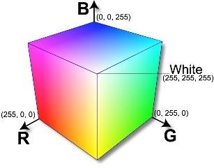
Most pixel-based image editors work using the RGB color model, but some also allow the use of other color models such as the CMYK color model. Nevertheless, the RGB color model is one of the most widely used color representation method in computer graphics as it uses a color coordinate system with three primary colors: red (R), green (G) and blue (B), where each of these colors can take an intensity value ranging from ‘0’ (lowest) to ‘255’ (highest). However, mixing these three primary colors at different intensity levels produces a variety of colors, as the collection of all the colors obtained by such a linear combination of red, green and blue forms the cube shaped RGB color space as in Fig. 3 [8][9].
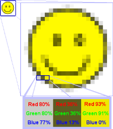
Figure 2. How each pixel has different color values in raster images.
Figure 3. A diagram showing the RGB color space [10].
- Image Pre-processing
 Pre-processing is a popular name for the operations performed on images for further use. However, image gray-scaling and image binarization, which both will be discussed in the following, are examples of these operations, as the aim of this type of operations is the improvement to the image data that suppresses unwilling distortions or enhances some image features that are important for further processing [11].
-
- Image Gray Scaling:
‘A grayscale (gray level) image is a simple digital image in which the only colors are shades of gray. Actually, the gray color is one in which all the components of red, green and blue have equal intensity in RGB space. Therefore, it carries only intensity information for each pixel’. Meanwhile, the process of converting a color image to a grayscale image is called gray scaling. However, to grayscale an image you should go through every pixel in the image calculating the average of the RGB channels’ values of that pixel, then you should assign each channel of the RGB with the resulting average value. An example of a color wheel image and its equivalent grayscale form is shown in Fig. 4 [12].
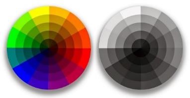
Figure 4. A color wheel and its grayscale form.
-
- Image Binarization:
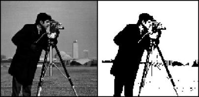
‘A binary image is a digital image which pixels have only two possible intensity values, which are normally displayed as black and white. Numerically, the two values are often 0 for black, and either 1 or 255 for white’. By and large, the color used to represent the object in the image is the foreground color, while the color that represents the rest of the image is the background color. Thus, the process of converting an image to a binary image is called binarization. However, to binarize an image it must first be converted to a grayscale image, and then by applying a specific threshold value on the image, all pixels will undergo a test that determines whether the pixel should be black or white, depending on that threshold value. An example of a grayscale image and its equivalent binary form is shown in Fig. 5 [12].
Figure 5. A grayscale image and its equivalent binary form.
In general, the threshold value is adaptive for each image and can be determined using one of the clustering algorithms (e.g., Otsu’s Method, Feng’s Method, Gatos et al.’s Method and Darek Bradley’s Method). However, we have chosen Otsu’s Method as our clustering algorithm, due to its speed and ability to handle different histograms of images. Consequently, after binarizing the image, the program will turn the image into an equivalent two-dimensional array of zeros and ones, where a zero refers to black (0) and a one
refers to white (255). In any case, the reason behind this operation is to simplify the process of manipulating and dealing with the image pixels in the following phases, considering that dealing with only one of the three RGB channels’ values is much easier than dealing with all of them. Subsequently, the resulting two-dimensional array that represents the binary image will make the program able to segment the image into separate components.
- Image Segmentation
Briefly, image segmentation is the identification of regions of interest in the image. In other words, it is the process of partitioning the image into a collection of images of the components that are suspected to be characters of a license plate, which later need to be recognized and saved as text. However, to achieve image segmentation, we have gone across two approaches.
-
- Horizontal and Vertical Projection:
This method handles the segmentation of the binary image by scanning the image array in two ways. Knowing that the characters in the image are arranged in the form of line(s), we are trying to determine the top and bottom edges of each line to obtain the parts of images that represent each line independently. In such a manner, the first way was to scan the image row-by-row, looking for a foreground row – a row that has black (foreground) pixels (columns) – that refers to the top edge of the first line of characters. At that instant, it starts copying the next rows’ pixels (columns) in a new image array starting from that row and, in the same time, keeps looking for a background row – a row whose pixels (columns) are all white (foreground) pixels – until it finds one. However, when it finds a background row, it stops copying and starts looking for another foreground row, to do the same thing until it reaches the last row in the image. Fig. 6 shall illustrate the process of obtaining the images of character lines.
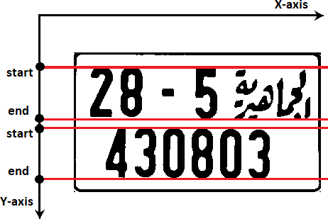
Figure 6. An illustration of the horizontal projection.
The second way was to obtain each individual character’s image by going through each “line image” column-by-column, looking for a foreground column that refers to the left edge of the character. However, when it finds a foreground column, it starts copying the next columns’ pixels in a new image, starting from that column, as it keeps looking for a
background column at the same time until it finds one. However, when it finds a background column, it stops copying and starts looking for another foreground column to do the same thing until it reaches the last column in the current “line image”. Fig. 7 illustrates the process of obtaining images of characters.
Figure 7. An illustration of the vertical projection.
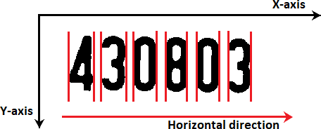
As a result, we expect to obtain a set of images, each of which containing one of the characters and ready for the next phase (the recognition phases).
The main advantage of this method is that it keeps the original ordering of characters, which is resulting from the horizontal and vertical scanning. Overall, the Horizontal and Vertical Projection method was thought to be a good solution for the segmentation problem, although we faced several issues while trying to implement it. One of these issues was the plate border issue, where a plate image usually contains a border outlining all the image boundaries, which may not be helpful for the horizontal/vertical projection. Therefore, we tried trimming the unwanted border parts from the image; however, the trimming solution was unsuccessful because of different plate forms and different sizes of the images that the program might cope with. In addition, the other issue was the smudge issue, where a smudge of mud or dirt on the plate might connect two lines/characters together, leaving no “background row/column” between them. Therefore, we decided to leave this method, and start looking for another approach to segment the plate image.
-
- Connected Component Labeling:
While we were searching and trying to come up with another approach to segment the image, we found what is known as the Connected Component Algorithm, which can be optimally used for such a task. However, a connected component is a set of connected pixels that share a specific property. In other words, the two pixels (p and q) are said to be connected, if there is a path of pixels with the same property from the first pixel (p) to the second one (q), where a path is an ordered sequence of pixels such that any two adjacent pixels in the sequence are neighbors. Accordingly, a component-labeling algorithm finds all connected components in an image and assigns a unique label to all points in the same component [13].
An illustrative example in Fig. 8 shows the result of labeling components in a simple (11×13) image using the Connected Component Labeling algorithm.
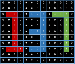
Figure 8. An example of the result of Connected Component Labeling.
The two approaches that can be used to implement the Connected Component Labeling are the recursive algorithm and the sequential algorithm. The recursive algorithm is quite straightforward. Nevertheless, it is inefficient, as the time taken by the algorithm increases rather quickly when the image size increases. Thus, we will not get into the details of this approach. On the other hand, the sequential algorithm consists of two passes. In the first pass, the algorithm goes through each pixel, checking the pixel above the current pixel and the one to the left of the current pixel, and in the same time, it assigns a label to the current pixel depending on the label value of these (previously labeled) pixels. In the second pass, it starts over from the very first pixel, and cleans up any mess it might have created in the previous pass, such as multiple labels for the same region (component) [14].
Although, the typical CCA that we have found also had a few issues, the main issue of the typical CCA was the ordering issue, where the components obtained from the CCA might not be in the right order. In other words, the CCA might lose the original ordering of the plate characters, which may not be helpful in recognizing license plate characters. Fig. 9 will show how the CCA could lose the original ordering of the characters.
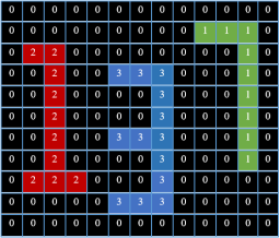
Figure 9. An example of the unordered CCA labeling result.
As you may have noticed, the peak of character ‘7’ is higher than the peak of character ‘1’. Therefore, character ‘7’ was labeled before character ‘1’ and was given a smaller label than the one given to character ‘1’. Nonetheless, according to the original ordering of the image characters, character ‘1’ should come first and then comes character ‘3’ and finally character ‘7’. Keeping in mind that a real plate image would have a huge number of pixels where the differences between the character peaks would not be noticeable as the ones shown in fig. 9. However, we succeeded in finding a good solution for this issue, which is going to be explained in details.
For the ordering problem, we suggested adjusting the algorithm in a way that maintains the original ordering of the plate characters. To illustrate more, this modification is based on sorting the components of the image depending on the coordinates of these components, where the algorithm obtains the coordinates of the first composing pixel of each component (the first pixel of each label) to keep these coordinates associated to their labels. However, before the beginning of the sorting process, it checks whether the input plate image was a rectangle-like or a square-like image. In case it was a rectangle-like image, it means that this image has only one line of characters/numbers. In the other case, when it is a square-like image, it finds that this image contains two lines of characters/numbers and has to be divided into two parts, an upper part, and a lower part, where each part should contain a single line of characters/numbers. Consequently, when the image is rectangle-like, the algorithm checks the horizontal coordinates for each component (label) in the image, and sorts these components depending on their horizontal coordinates. As shown in fig. 10, the horizontal coordinates get higher as they move towards the right, and since characters are arranged from left to right, the leftmost character is the first one, followed by the next character/s on its right side. On the whole, when the sorting process is finished, the algorithm would obtain a sorted list of all the components (labels) as shown in fig. 11.
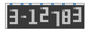 Figure 10: An example of a simple rectangle-like plate image.


Figure 11. The sorted list of components of the image shown in fig. 10.
As you can see in fig. 11, label ‘3’ would go first in the sorted list, label ‘7’ would be the second and so on. Overall, sorting the components depending on their horizontal coordinates would work perfectly on the rectangle-like plates. However, when it is a square-like plate, the algorithm, as mentioned before, must first split the image array into two separate parts, an upper part, and a lower part, and then sorts both parts as if they both were rectangle-like images. The upper part goes from the beginning of the image (the first row) to middle of the image (image height/2), while the lower part starts right after the middle of the image until the end of the image (the last row) as illustrated in fig. 12. In any case, each part would be treated independently, and when the process of sorting the components for both parts finishes, the algorithm combines the components of each part in a single sorted list containing the components of the first (upper) part followed by the components of the second (lower) part.
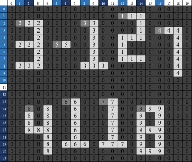
Figure 12. An example of a simple square-like plate image.
The reason behind splitting the square-like image array into two parts is that this plate image has two lines of characters/numbers, where the characters (components) of these lines share the same horizontal coordinates. Therefore, they cannot both be sorted in the same image array. As shown in the fig. 13, the upper part labels would be sorted from label ‘2’ to label ‘4’ and followed by the labels of the lower part from label ‘8’ to label ‘9’.
Figure 13. The sorted list of components of the image shown in fig. 12.
Furthermore, there was a issue with some of the English characters such as (K, V, W, X and Y), where the CCA fails to label the components representing these characters with only one label, due to the top right edge that exists in all of these characters. Fig. 14 shows an example of this issue with the English letter ‘Y’ as a connected component.
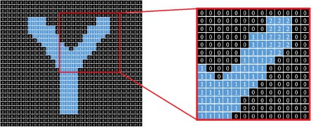
Figure 14. The ‘Y’ letter as a connected component after the first pass.
Fig. 14 shows the problem that the CCA faces when labeling the letter ‘Y’ as a component, where all the labels (2, 3, 4, 5 and 6) should be changed to ‘1’ in the second pass of CCA so the component of interest would only have one label after the second pass. However, the labels ‘1’ and ‘2’ did not have the chance to meet in the first pass. Therefore, they were not compared to one another; accordingly, the dictionary (Hash Map) did not have label ‘2’ as a value to the key ‘1’ to correct it in the second pass. As a result, the output of the second pass would be as shown in fig. 15.
Figure 15. The letter ‘Y’ component facing the top-right edge issue after the second pass.
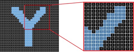
As shown in fig. 15, the CCA fails to label the letter ‘Y’ properly. In fact, it fails to label all the letters that have the same top right edge as in the letters (K, V, W, and X). Overall, as long as the Libyan license plate does not contain any English letters this issue will not be our biggest concern at present. Although, we did attain a good solution to this issue, which is going to be explained in details. For the top-right edge issue, we suggested adding a couple of passes after the original two passes of the CCA are finished. In the so-called ‘third pass’, the algorithm is going to work on scanning the image array and repeating only a part of the first pass, where it will look for all the non-zero pixels that have two non-zero neighbors with different labels, compare the labels (numerically), and finally assign the minimum label to the current pixel. Regularly, based on the comparison result, a new piece of information is added to the dictionary (Hash Map) that will be used in the next pass. Finally, the last pass is exactly the same as the second pass of the CCA, where the algorithm calls the function that implements the second pass again after finishing the newly created ‘third pass’, owing to correct any false labeling that might have occurred. Overall, the result of this repetition is labeling all the components appropriately, including the components that represent characters that have a top-right edge.
Optimistically, this modification would work well for all the Libyan license plates, in addition to all the plates that have the same dimensions and the same structure. In this way, the CCA would work well for segmenting the image into separate components, as well as maintaining the original ordering of these components.
- Image Classification
Image classification is the process of marking images with particular predetermined categories. It is done with the help of image pre-processing, image sensors, object detection, object segmentation, feature extraction and object classification. Meanwhile, there are several classification techniques for image classification, e.g., Artificial Neural Networks, Decision Trees, Support Vector Machines and Fuzzy Classification [15]. In this work, we have utilized Google Brain’s TensorFlow classifier for the classification process, which is an open-source software library for high-performance numerical computation. It was originally developed by engineers from the Google Brain team within Google’s AI organization, as it was meant for different types of perceptual and language understanding tasks [16]. However, we have only used a few classes from the TensorFlow library, which are specialized in character recognition, where some of these classes are used for training the classifier, while others are used for the classification (recognition) process itself. On the whole, the proposed algorithm for the suggested modification of the typical CCA is as follows.
- Start.
- Load image file.
- Do pre-process.
- Convert image to an array.
- Label connected components.
- If the image is rectangular (Yes: go to step No.8), (No: continue).
- Split into two parts.
- Sort image(s) characters.
- Save characters.
- Recognize characters.
- Output text.
- Stop.
- Implementation and Results
- Implementaion
Using what was previously introduced, and according to the designed algorithm, the implementation will be carried out through a series of steps as follows:
-
- Image File Loading: The first step is finding a way to take an image file in a readable data format as an input to the program, which was done using Java’s Image Library. Fig. 16 will show the plate image that we are going to take as an example.
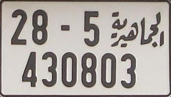
Figure 16. An example of a square-like Libyan plate image.
-
- Image Preprocessing: After getting the input image file, the next step is to perform a few operations on the image to prepare it for the next phases. However, the first operation works on Grayscaling the image or turning the original color image into a grayscale image as shown in fig. 17, by calculating the average of the RGB channels’ values and assigning all the RGB channels with the resulting average to the current pixel.
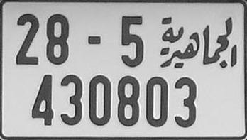
Figure 17. Turning the original color image into a grayscale image.
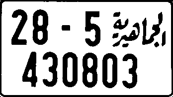
After obtaining a grayscale image, it should be turned into a binary image with the help of a specific threshold value that is determined by implementing Otsu’s binarization method. Thus, the result of binarizing the grayscale image is shown in fig. 18.
Figure 18. Result of binarizing the grayscale image.
-
- Convert the Image to an Array: Since all the RGB channels’ values of each pixel are of the same value, the obtained binary image should be turned into an equivalent two-dimensional integer array of 0s and 1s. Where ‘0’ refers to black (0) and ‘1’ refers to white (255). Since the image array may have hundreds of thousands or even millions of pixels, it cannot be hypothetically represented in a single typical A4 page. Therefore, we will only try to show representations of a small part of the image array, hoping that it will illustrate the idea. Fig. 19 shows a hypothetical representation of how the character ‘2’ is going to be represented in the real image array.
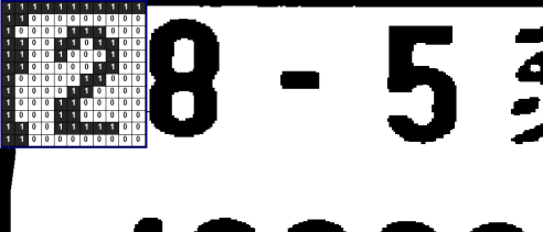
Figure 19. A representation of a part of the image array. Figure 19. A representation of a part of the image array.
The resulting two-dimensional array that represents the binary image, as illustrated in fig. 19, will make the program able to segment the image into separate components.
-
- Labeling and Sorting Connected Components: As mentioned before, segmenting the image into a set of components requires labeling each component with a unique label as in fig 20. Therefore, the modified CCA that was suggested earlier should handle the labeling process.
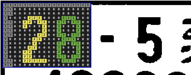
Figure 20. A simple representation of the result of labeling connected components.
After labeling every component in the image array, we added a simple operation that could help to get rid of the components that are too small to be characters as well as the components that are too big. The operation removes all connected components that have less than a certain number of pixels or more than a certain number of pixels based on the plate image size. Next, the program should check if this image was a square-like image or not, where a square-like image should be divided into two horizontal parts as mentioned in the modified CCA. After that, the program is going to sort the components according to their horizontal coordinates in order to obtain a sorted list of all the image components to be able to segment and save the characters’ images in the right order during the next step.
-
- Saving the Characters: Saving the components’ (characters’) images after finishing the labeling and sorting process requires determining the height and the width of each component to create an image with the appropriate dimensions for all the components in the image, in addition to copying each component’s pixels in its own newly created image. Determining the height and width of the components is done by scanning the image while seeking the first pixel that has the value of each label in the order of the sorted list of labels. However, when the program finds the first pixel of the first label, it loops through all the pixels containing that label, looking for the highest and lowest points (pixels) for both horizontal and vertical coordinates. Successively, it subtracts the lowest point (index) from the highest point of the horizontal and vertical coordinates, in order to determine the dimensions of that component to create an image object with the same dimensions. Consequently, the newly created image’s pixels are going to be filled with the component’s pixels to obtain an image that contains only this single component (character). Regularly, the same thing should go for all the remaining labels (components) in the image. Fig. 21 shows how some of the characters of the plate image would appear after the segmentation process.
Figure 21. An example of the segmentation phase result.
However, since the TensorFlow classifier requires specific dimensions for input images, we should adjust the output size of the segmented images before sending them to the classification phase. Therefore, images need to be resized to specific dimensions as the library requires, which are 200 pixels in both width and height, to create the image file before saving it in the specified directory. For illustration, Fig. 22 shows the actual results of the segmentation phase.
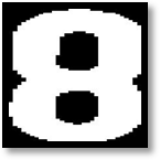

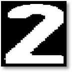
Figure 22. The result of the segmentation process.
-
- Classification and Character Recognition: obtaining only the containing image of each character is not enough, where a classifier must be used to recognize the images obtained from the segmentation phase. As mentioned before, the TensorFlow classifier will be used in the classification process, as it must be provided with abundant, real, and adequate data to be able to give accurate and correct results. Nevertheless, after finishing the image segmentation phase, the program is going to apply the classification process to recognize the obtained components, and give the desired results by using the classifier that was provided with the required data and trained properly. Noting that both the amount of data and the training rate of the classifier have a great impact on the accuracy of the recognition process. Finally, the program will show the text obtained from the classification process.
- Results


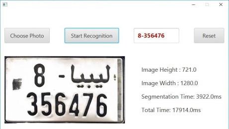
 Through what was previously introduced about the implementation of the software application, we can say that we have attained some fascinating results, as we consider those results doubtlessly beneficial for this particular case study, which is the recognition of characters of Libyan license plates. In any case, Fig. 23 shows the result of segmenting and recognizing characters of a Libyan license plate, as well as the time taken to segment the image (segmentation time), accompanied with the time of the whole process (total time) including the classification phase time.
Figure 23. The user interface of the software application.
Based upon that, fig. 24 is going to show a table of different license plate forms, and an illustration of the segmentation process and the average time of segmenting each character. In addition, it is going to show how the output would look like and how it is going to change before it goes as an input to the recognition phase. Finally, it displays what results were obtained, each of which combined by an accuracy percentage.
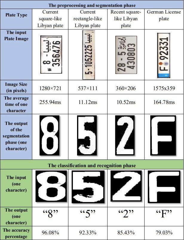
Figure 24. Results of recognizing characters from different license plates.
- Conclusion
We believe that this work is considered as an “added value” to the scientific researches in this field, where the proposed algorithm has presented actual set of solutions for recognizing
characters from license plates. Keeping in mind that the outputs of applying this algorithm represent a treasure in the form of text for many governmental and non-governmental applications. In addition, this system can also be adjusted in a way that makes it capable of recognizing characters from paper documents. However, although it is possible to prepare the system for dealing with most types of plates, the license plates of vehicles in the United States of America are a bit difficult to recognize, because the background of the characters in U.S. license plates may contain different shapes and colors that could make the process more complicated. Regardless, we believe that the design of this algorithm is imperfect and upgradable as we intend to improve it in the future, where it can be optimized to perform the “plate localization phase”, which takes an image of a car on the road and locate the plate image as a first step before processing the image. Furthermore, other image preprocessing techniques can also be added to the algorithm (e.g. image skewing, image rotation, and image enhancement techniques) to make it capable of handling images of crooked plates as well as coping with low-resolution images.
Overall, we are optimistically looking forward to accomplishing these improvements as well as overcoming these limitations in the near future.
References
- Sousanis J. (2011). World Vehicle Population Tops 1 Billion Units [ONLINE]. Wardsauto. Available at: https://www.wardsauto.com/news-analysis/world-vehicle- population-tops-1-billion-units (Accessed: 1 August 2018).
- Kawade S., Mukhedkar M. (2013). A Real Time Vehicle’s License Plate Recognition System [ONLINE]. International Journal of Science and Engineering. Available at: https://pdfs.semanticscholar.org/1a79/798226c044f50f9b7e802940 67ac3397a28c.pdf (Accessed: 17 August 2018).
- Grant J., (2010). Automatic License Plate Recognition [ONLINE]. Department of Computer Science and Engineering,
- University of Notre Dame. Available at: https://www3.nd.edu/~jgrant3/cw/alpr.pdf (Accessed: 23 August 2018).
- Girod, B. (2018). Digital Image Processing [Online]. Stanford. Available at:
- https://web.stanford.edu/class/ee368/Handouts/Lectures/2019_Win ter/1-Introduction.pdf (Accessed: 21 August 2018).
- Blinn, J.F., (2005). What is a pixel. IEEE computer graphics and applications, 25(5), pp.82-87.
- Scholarspace. (2019). All About Images [ONLINE]. Research guides. Available at: https://guides.lib.umich.edu/c.php?g=282942&p=1885352 (Accessed: 21 August 2018).
- Vector Conversions. (2019). Vectorising [ONLINE]. Raster vs Vector. Available at: https://vectorconversions.com/vectorizing/raster_vs_vector.html (Accessed: 5 September 2018).
- HP Development Company. (2018). Tech takes [ONLINE]. Print Basics: RGB VersusCMYK. Available at: https://store.hp.com/us/en/tech-takes/print-basics-rgb-vs-cmyk (Accessed: 5 January 2019).
- Geeks for Geeks. (2017) Computer Graphics, The RGB color model [ONLINE]. Available at:https://www.geeksforgeeks.org/computer-graphics-the-rgb-color- model/ (Accessed: 5 January 2019)
- Santosh Dahal. (2016) What is Image [ONLINE]. Available at: https://www.suntos.com.np/computer-vision-for-robotics/what-is- image.html (Accessed: 3 January 2019).
- Sonka, M., Hlavac, V. and Boyle, R., 1993. Image pre-processing. In Image Processing, Analysis and Machine Vision (pp. 56-111). Springer, Boston, MA.
- Songke Li, Yixian Chen, 2011, License Plate Recognition, p. 5-6.
- Ramesh, J. (2003). Computer Vision [ONLINE]. University of Nevada, Reno. Available at: https://www.cse.unr.edu/~bebis/CS791E/Notes/ConnectedCompon ents.pdf (Accessed: 21 August 2018).
- Sinha, U. (2018). AI Shack. [ONLINE]. Labeling Connected Components Available at: http://aishack.in/tutorials/labelling- connected-components-example (Accessed: 10 January 2019).
- Kamavisdar, P., Saluja, S. and Agrawal, S., 2013. A survey on image classification approaches and techniques. International Journal of Advanced Research in Computer and Communication Engineering, 2(1), pp.1005-1009.
- Tensorflow. (2017). About TensorFlow [ONLINE]. Available at: https://www.tensorflow.org/. (Accessed: 1 February 2019).
- Eslam Eldharif (2018). Solving the Problems of Timetable Using Genetic Algorithm Case Study: Faculty of Information Technology Timetable.
