
Mohammed. A. Elbargthy1, Nasir Elmesmari2*, Mohammed Elnazzal3
1,3 Department of Statistics, Faculty of Science, University of Benghazi, Benghazi, Libya
2 Department of Statistics, Faculty of arts and Science, Al Maraj, University of Benghazi, Benghazi, Libya
Correspondent Email: nasir.elmesmari@uob.edu.ly
HNSJ, 2024, 5(3); https://doi.org/10.53796/hnsj53/21
Published at 01/03/2024 Accepted at 20/02/2024
Abstract
This study is an attempt to find a more adequate model for the celebrated Canadian lynx data (1821 – 1934) than the classical models suggested by other researchers mentioned in the literature [Campbell and Walker (1977)]. In the previous in which studies the logarithmic transform to base 10 was used, in this study both logarithmic and square root transforms are used for the sake of comparison. Our results seem to suggest that the models fitted using logarithmic transformed data are in general superior to their counterparts under the square root transformation in terms of the significance of parameter estimates and their standard errors. The classical model ARMA (3,3) and our own model ARMA (3,0) were found to provide a reasonable model to logarithmic transformed lynx data.
Key Words: Canadian Lynx data, The logarithm and square root transformation, ARMA (3,3), ARMA (3,0).
المستخلص
هذه الدراسة عبارة عن محاولة لايجاد نموذج أكثر ملائمة من النماذج المقترحة في الدراسات السابقة لبيانات حيوان الوشق الكندى. ففى الدراسات السابقة النموذج المقترح هو تحويلة اللوغاريتم الطبيعى للاساس 10، أما في هذه الدراسة تم اقتراح تحويلة الجذر التربيعى ونموذج الانحدار الذاتى للرتبة 3 ARMA(3,0) حيث اظهرت النتائج أن اداء نموذج تحويلة اللوغاريتم الطبيعى يفوق اداء نموذج الجذر الترببيعى بينما لا يوجد أختلاف بين نموذج تحويلة اللوغاريتم الطبيعى للاساس 10 ونموذج الانحدار الذاتى للرتببة3 ARMA(3,0).
1. Introduction
A time series (TS) is a sequence of observations of one variable ordered in time. These observations are collected at equally spaced, discrete time intervals. Although in some cases the ordering may be according to another dimension. The measurement of some particular characteristic over a period of time constitutes a time series. It may be an hourly record of temperature at a given place or a quarterly record of gross national product. A time series is regarded to be continuous when observations are made continuously in time, also it is regarded to be discrete when observations are taken only at specific time usually equally spaced. [Anderson, T. W (1971)].
A stochastic process is a family of real valued random variables where subscripts refer to successive time periods, and is denoted with Each of the random variables in the stochastic process has generally its own probability distribution and are not independent. Consider that for each time period we get a sample of size one (one observation) on each of the random variables of a stochastic process. Therefore, we get a series of observations corresponding to each time period and to each different random variable. The special feature of time series data is the fact that successive observations are usually not independent, and the analysis must take into account the time order of observations.
1.1 Collection Time Series Data
We will discuss the importance of data and data collection, components of time series data, graphical presentation of data, and numerical presentations and transformations of time series data. Each of these procedures will be important in building our tools for time series analysis and forecasting methods. And where the first and one of the most important steps in the analysis of time series data and the subsequent development of a forecasting model is the collection of valid and reliable data. Analysis and forecasting are no more accurate than the data used to generate summary statistics and forecasts. The most sophisticated statistical techniques and forecasting model will be useless if applied to unreliable data. [Gaynor P.E. and R.C. Kirkpatrick (1994)]
1.2 Nonstationary Process
If we have assumed that underlying process is stationary, this implies that the mean, the variance, and auto covariance of the process are invariant under time transformations. Thus, the mean and the variance are constant, and the auto covariance depends only on the time lag. Many observed time series, however, are not stationary. In particular, most economic and business series exhibit time-changing levels and/or variances. A changing mean can often be described by low-order polynomial in time. However, frequently the coefficients in these polynomials are not constant but vary randomly with time. Such nonstationary, in which the observations are described by random (or stochastic) trends, is usually referred to as homogeneous nonstationary. It is characterized by a behavior in which, apart from local level and/or local trend, one part of the series behaves like the others.
1.3 Stationarity Process
In order to analysis time series a good number of stochastic models have already been developed, a central feature in the development of time series models is an assumption of some of statistical equilibrium. An important class of stochastic models for describing time series is called stationary models, which assume that the statistical properties of the process do not change over time. Usually, a stationary time series can be usefully described by it is mean, variance and autocorrelation function. A process with approximate constant mean, variance and autocorrelation through time is called a stationary process. [Box-Jenkins, (1970)].
1.4 Autoregressive Process of Order p [AR(P)]
The process is said to be an autoregressive process of order p; if it satisfies the difference equation:
Where are constants and a purely random process (white noise). [Pristely, (1981)].
1.5 Moving Average Process of Order q [MA (q)]
The process is said to be a moving average process of order q if it can be written as
where are constants and is a stationary purely random process.
Note that we may, without any loss of generality, assume that or .
It is clear that we cannot assume that ( or ) simultaneously. Since is a linear combination of uncorrelated random variables it is easy to see that is always a stationary process. It is sometimes useful to express a moving average process in autoregressive form. If this is to be done; the moving average parameter must satisfy the invariability condition which takes a form similar to that which has to be imposed on autoregressive to ensure stationarity. The autocorrelation function MA(q) cuts of after lag q (i.e. = 0; k > q); while the partial autocorrelation function is infinite in extent and dominated by damped exponentials.
The used in constructing both the (AR and MA) process, but the difference between the two types of processes is that, in AR case is expressed as a finite linear combination of its own past values and the current value of . [Pristely, (1981)].
1.6 Mixed Autoregressive Moving average process [ARMA(p,q)]
Mixed autoregressive and moving average process having p-AR and q-MA terms, is given by:
Where and are a constants and is a purely random process; and denoted by ARMA ( p,q ).
For an ARMA process to be stationarity we have to assume that the roots of are outside the unit circle and for invariability we have to assume that the roots of are outside the unit circle.
Many obvious advantages arise in using ARMA models which combine terms of both the AR and MA type, and in fitting models to observational data it is often possible to fit an ARMA models of smaller order than would be required in purely AR or MA models. [Fuller, (1976)].
2. The Lnx Data
The Canadian lynx data set is the annual record of the number of the Canadian lynx “trapped” in the Mackenzie River district of the North-West Canada. These data are actually the total Fur returns, or total Fur sales, from the London archives of the Hudson’s Bay Company in the years of 1821–1891 and 1887–1913; and those for 1915 to 1934 are from detailed statements supplied by the Company’s Fur Trade Department in Winnipeg; those for 1892–1896 and 1914 are from a series of returns for the MacKenzie River District; those for the years 1863–1927 were supplied by Ch. French, then Fur Trade Commissioner of the Company in Canada. By considering the time lag between the year in which a lynx was trapped and the year in which its fur was sold at auction in London, these data were converted in Elton and Nicholson (1942) into the number that were presumably caught in a given year for the years 1821–1934 which giving a total of 114 observations.
3. Previous Studies
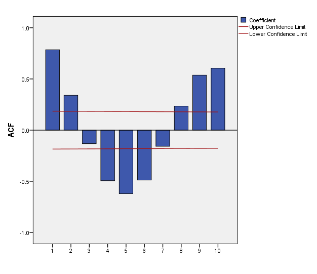
In 1953 P.A.P. Moran suggested that the logarithms transformation is an optimal solution for the Canadian lynx data. Since Moran noticed a damping in the sample correlogram then he made the first model for this data which is AR (2). Figure (1) shows the logarithms (to base 10) of the annual trapping of the lynx over the period (1821 – 1934), giving a total of 114 observations. This is a celebrated set of data and has been the subject of great deal of study among time series analysis by Campbell and Walker (1977) who gave an interesting review of previous analyses. The dominant feature of the graph is that the data contain persistent oscillations with a steady period of approximately ten years, but with irregular variations in amplitude. The sample autocorrelation function is shown in figure (2), where the strong periodic behavior of this function confirms the “Pseudo periodicity” in the data. However, the autocorrelation also shows some degree of damping, which is consistent with the irregular variations of amplitude in the data. The form of both the data and the autocorrelation function suggests that there is a strictly periodic component corrupted by “error”, alternatively that the data conform to some “pseudo periodic” type of ARMA model. The former type of model is that chosen by Campbell and Walker (1977). The above account on the lynx data was taken almost literary from Priestley (1981, p384).
Figure 1: the logarithms (to base 10) of the lynx data over the period (1821 – 1934)
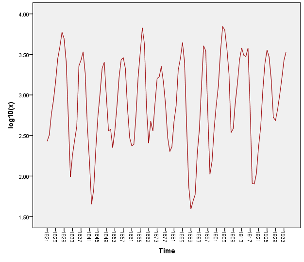
Figure 2:The sample autocorrelation function of logarithms the data
4. Methodology
In many aspects of time series analysis, data transformations are useful, often for stabilizing the variance of the data. Non constant variance is quite common in time series data. A very popular type of data transformation to deal with non-constant variance is the Power family of transformations. given by:
Where is the geometric mean of the observations ]}. If , there is no transformation. Typical values of used with time series data are (a square root transformation), (the log transformation), (reciprocal square root transformation), and (inverse transformation). The divisor simply a scale factor that ensures that when different models are fit to investigate the utility of different transformations (values of ), the residual sum of squares for these models can be meaningfully compared. The reason that implies a log transformation is that ( ) approaches the log of x as approaches zero. Often an appropriate value of is chosen empirically by fitting a model to for various values of and then selecting the transformation that produces the minimum residual sum of squares. The log transformation is used frequently in situations where the variability in the original time series increases with the average level of the series. When the standard deviation of the original series increases linearly with the mean, the log transformation is in fact an optimal variance-stabilizing transformation. The log transformation also has a very nice physical interpretation as percentage change [Montgomery 2008]. When the data has exponential growth, the optimal transformation is taking the logarithm of the values which called (log transform). The problem with protentional curve that is the growth rate not clear how much would be.
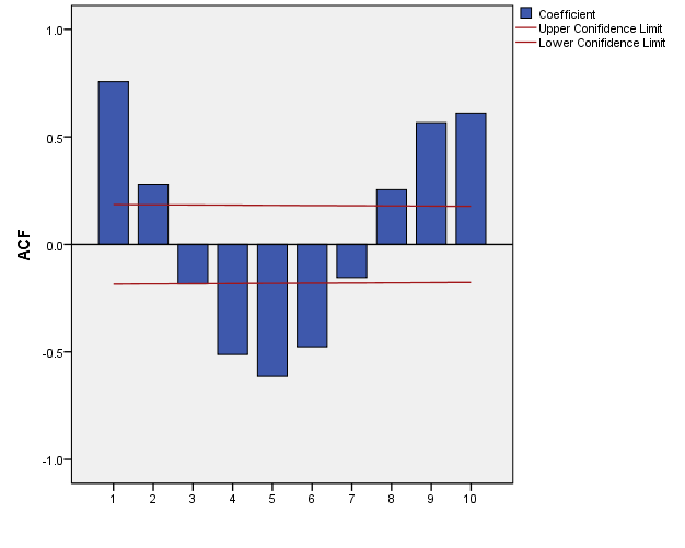
As far as the lynx data under square root is concerned, to our knowledge no attempt was made to study its correlation structure under this transformation. The square root transformed lynx data is plotted in figure (3) with its sample autocorrelation function in figure (4).
Figure 3: the square root of the lynx data over the period (1821 – 1934)
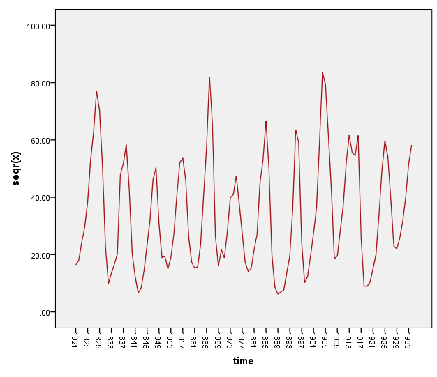
Figure 4:The sample autocorrelation function of square roof of the data
5. Analysis
The ARMA models of order ARMA (3, 3) and ARMA (3.0) under both transformations (the logarithm to base 10 and square root) were fitted to the lynx data. The results are given in tables (1 and 2) which include: parameter estimates, standard errors, calculated p-values, p value for Ljung Box test, stationary R square, normalized Bayesian information criterion (BIC), root mean square error (RMSE), mean absolute percentage error (MAPE).
Table 1:The results of the fitted ARMA(3,3) model under both transformations
| Estimates | The logarithmic transformed | The square root transforms |
| constant | 2.906 | 34.144 |
| SEP-Value | 2.0830.127
0 |
1.9960.006
0 |
| SEP-Value | -1.7850.201
0 |
-1.6470.006
0 |
| SEP-Value | 0.4990.124
0 |
0.4070.003
0 |
| SEP-Value | 0.9050.123
0 |
0.9470.098
0 |
| SEP-Value | -0.0990.144
0.493 |
-0.0280.124
0.825 |
| SEP-Value | -0.4900.102
0 |
-0.5910.104
0 |
| P-value Ljung Box test | 0.055 | 0.124 |
| R-Square | 0.864 | 0.837 |
| BIC | -2.813 | 4.472 |
| RMSE | 0.212 | 8.090 |
| MAPE | 6.166 | 21.846 |
Table 2:The results of the fitted ARMA(3,0) model under both transformations
| Estimates | The logarithmic transformed | The square root transforms |
| constant | 2.903 | 34.127 |
| SEP-Value | 1.2870.095
0 |
1.2640.095
0 |
| SEP-Value | -0.5770.146
0 |
-0.6280.142
0 |
| SEP-Value | -0.1180.095
0.220 |
-0.0630.096
0.515 |
| P-value Ljung Box test | 0.006 | 0.011 |
| R-Square | 0.832 | 0.792 |
| BIC | -2.755 | 4.564 |
| RMSE | 0.232 | 9.015 |
| MAPE | 6.834 | 27.918 |
Figure 5:The residuals series of ARMA(3,3) model
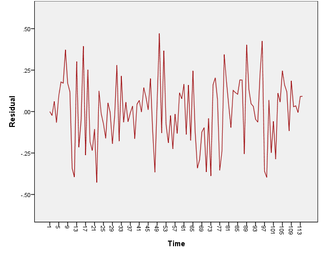
Figure 6:The residuals series of ARMA(3,0) model
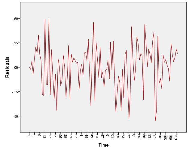
Figure 7:The autocorrealtion function of residuals series for ARMA(3,3) model
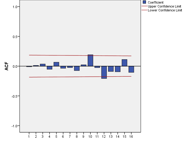
Figure 8:The autocorrelation function of residuals series for ARMA(3,0) model
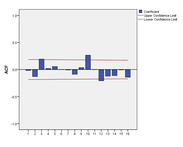
Figure 9:Histogram of residuals series for ARMA(3,3) model
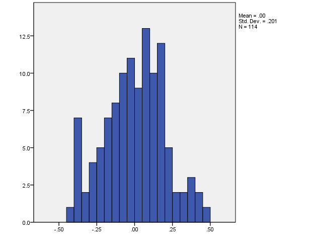
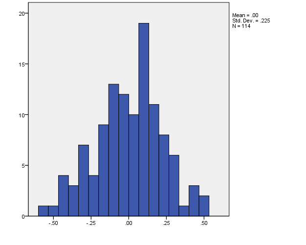
Figure 10:Histogram of residuals series for ARMA(3,0) model
6. Discussion and Conclusion
The results in tables (1 and 2) seem to suggest that the models fitted under logarithmic transformation are in general better than their counterpart models fitted under square root transformation. The Lujng box failed to give non-significant results (p > 0.05) accepting the randomness especially ARMA (3,0) model. The two models ARMA (3,3) which among the classical models mentioned in previous studies in the literature and our own model ARMA (3,0) seem to be plausible models, because it appears that they satisfy the first stage indication of a good model where parameter estimates are significant except one parameter estimate in the case the ARMA (3,3) model. The values of R square, RMSE, MAPE and normalized BIC are slightly smaller in the case of the ARMA (3,3) model than in the ARMA (3,0) model case. ARAM (3,3) model under logarithmic and square root transformation give non-significant results for Lujng-Box test which means that the assumption that the errors are white noise cannot be rejected, whereas in ARAM (3,0) model the errors term did not pass the test. However, the plots of series, autocorrelation function, and histogram of the residual for both models indicate the randomness of the errors where no apparent trend (figures 3 – 10).
References
|
|
|
|
|
|
|
|
|
|
|
|
|
|
|
|