
PERFORMANCE ANALYSIS OF QUEUING AND COMPUTER NETWORKS
Aimen Abdalsalam Kleep1, Ashrf Ali Nasef2, Salem Husein Almadhun3, Aimen M. Rmis4, Ali Muftah Benomran5
1 Department of Computer, Faculty of Education, Elmergib University, Al Khums, Libya;
2 Department of Computer Science, Faculty of Science, Alasmarya Islamic University, Zliten, Libya; ashrfnasef@asmarya.edu.ly
3 Department of Computer, Faculty of Education, Elmergib University, Al Khums, Libya;
salem.almadhun@elmergib.edu.ly
4 Department of Computer Science, Faculty of Science, Alasmarya Islamic University, Zliten, Libya;
5 Department of Computer Science, Faculty information technology, Alasmarya Islamic University, Zliten, Libya;
it.ali_bomran@asmarya.edu.ly
HNSJ, 2024, 5(7); https://doi.org/10.53796/hnsj57/17
Published at 01/07/2024 Accepted at 18/06/2024
Abstract
Queuing is one of the most usable tools that help in analyzing the performance of complex telecommunication and system networks. Thus, this term paper presents the performance measurements of computer networks with queuing technique. The paper covers the detail introduction of queuing theory and its various applications widely used for complex network/system environment.
Introduction:
Computer systems today, getting more advanced and modernized in features that causes more complexity in system/network environment. The rapid changes increased the demand of such tools that can help resolving and understanding such systems’ behavior (unknown, xxxx). Queuing is a popular tool that mostly use in the analysis of a robust systems and networks (B. Filipowicz & J. Kwiecień, 2008). The queuing theory mainly emphasizes on the most dreaded life events, such as waiting. Queuing is quite popular in various fields. They include computer systems, telephone conversations, in premises such as a petrol station and a supermarket among others (Dr. János Sztrik, 2010).
In a queuing system, inputs, queues, and servers act as service centers. In the recent decades, the queuing theory has become a subject of great interest to professionals such as Economists, Mathematicians, and Engineers (Filipowicz & Kwiecień, 2008). It mainly entails an advanced analysis of the features of queues using various mathematical models to develop solutions to some of the models that pose a real challenge to system/network analysts (Robertazzi, 2000).
A queuing system is made up of servers as service centers, inputs and queues. It is made up of more than one server whose task is to serve clients depending on their arrival time. The flow of entities is the customer who represents jobs, users, programs and transactions. They come to the service facility to receive a particular service. They may even have to wait in the waiting room in an instance where there are many customers in need of the same service. They leave once they receive an appropriate service. Unfortunately, some of the customers disappear in the system. There are various factors that describe the queuing system. These factors include the number of servers, the arrival intervals, discipline being served, distribution of the time of service, and maximum capacity among other factors (B. Filipowicz & J. Kwiecień, 2008).
The likely characteristics of the service time, the queue for requests, and the disciplines being served must be determined in order to categorize a queuing system. Conversely, the distribution of the customers’ entry times, represented as A (t), may be used to categorize the arrival process, as A (t) = P (inter-arrival time < t). Moreover, the analyst in the queuing theory makes the assumption that the inter-arrival periods are independent. Furthermore, the theory presupposes that they are equally distributed random variables. The other variable that is considered random is the service time. It is called a “service request” in certain contexts. This variable is represented by the distribution function B(x), that is, B(x) = P (service time < x). (Allen, 1990).
The number of servers is determined by a variety of criteria, such as the service discipline and the service structure that is being sought. The number of servers refers to the maximum population of customers that stay in a system including those that are being served at that particular moment. The discipline of the service dictates the regulations which are followed when choosing the next customer (Baloch .et, all, 2006). There are various queuing laws. They include:
First in First out (FIFO)
According to this rule, each order is completed depending on its arrival time. The order that arrives first receives service before those that arrive later. Hence, arrival time determines the time when an order will be served (Arnold O. Allen, 1992).
- Last in First Out (LIFO)
According to the rule, the order that is last in the queue is the one that is really released first. It is the antithesis of the first in, first out policy, even if a task is started as soon as it is delivered. A job may be started earlier, but the server may switch to other tasks for some time; thus, delaying the completion time of the earlier order (Arnold O. Allen, 1992).
- Time Sharing
This refers to an instance where the CPU performs one major task for a certain length of time. Once, it is done, it begins another task. The CPU may recycle the task; that is, it puts it into the queue so that whatever exercise remains are completed at a different time. The CPU repeats the process until all the tasks are completed (Adrian E. Conway and Nicolas D. Georganas, 1987).
- Orders for job queues
In a queue each tasks is executed at a particular time. Alternatively, it may be done through time sharing. In either of the alternatives, the order in which jobs are completed is important (Adrian E. Conway and Nicolas D. Georganas, 1987).
- Smallest job first (SJF)
In this protocol, the job orders are executed in terms of their size. This makes it possible to complete many jobs at a minimal time (Adrian E. Conway and Nicolas D. Georganas, 1987).
- Priority
According to this rule, a task is executed depending on the necessity and not arrival time. A personal computer is one of the devices that prioritize its operations a great deal. There is frequently a long queue filled with different events from different input devices, such the keyboard and mouse, among others. In such an instance, the PC may give the mouse a priority (Nico M. Van Dijk, 1995).
Computer systems experience queues on a regular basis. Some of the queues inquire waiting for a computer system to get processed, such as a queue of requests from the database, and I/O requests among others. It is important to note that a queue has only a single service facility. However, the server may be more than one, and a buffer of either an infinite or finite capacity (Trivedi, K., 2002).
Analyzing D/D queues is simple when compared to others. It is even simpler when the service and the inter-arrival time have fixed values. There are many features of such queues. They include the exponential service time, Poisson arrival process, and the relationship between arrival and service time. In the initial positions, it is denoted by M; that is, (M/M/ · /·). The Markovian queues have a less memory. Hence, they are amenable to analysis. The case is attributed to the fact that they are continuous chains with an exponential transition state (Moshe Zukerman, 2015). These applications are as illustrated below:
The D/D/1 queue
Take the following case into consideration λ > µ. In such an instance, the D/D/1 queue is deemed as being unstable. It grows on a regular basis towards its infinity t → ∞. The server remains busy as there are many packets in need of service. Hence, the utilization amounts to one (Moshe Zukerman, 2015).
Now, assuming that λ < µ, examine a stable D/D/1 queue. Take note that in the event that the arrival and departure times coincide for every D/D/1, the aforementioned assumption applies. If departure comes first, then λ = µ is likewise constant. Considering that time t=0 is the initial arrival. The arrival time of the service will end at t= 1/µ. The second arrival is scheduled for t = 1/λ, and it is serviced at t = 1/λ + 1/µ. When the queue size has two numbers, 0 and 1, this gives rise to the deterministic cyclic process. The representation of the transitions between time points 0 and 1 is n(1/λ), where n = 0, 1, 2,…
Conversely, n(1/λ) + 1/µ, where n = 0, 1, 2,…, represents the transition from 1 to 0 time points.
When a client is being serviced in a 1/µ time period, each cycle has a time period of 1/λ. During the interval 1/λ − 1/µ, no client is utilizing the service. Therefore, the use might be given by;
ˆ U = (1/µ)/(1/λ) = λ/µ.
A consumer receives service before the next one comes when they enter the system. According to Moshe Zukerman (2015), the mean size of a D/D/1 should thus be equal to the mean queue size of the server, which also means it is equal to use. There are many applications of a queue. Some of them include:
The M/M/1 Queue:
Customers in the M/M/1 Queue arrive according to the Poisson process, whose standard rate is λ. The time required to attend to each consumer is exponential r. v., where µ is the parameter. Therefore, it is thought that clients choose their exponential service time. Notably, the time of service is mutually independent. Moreover, it is independent of the arrival time. In an instance where a customer meets an empty system; he is served immediately. However, if the system is serving other customers, the new customer queues. When the customers have been served, they leave while another one from the queue receives the service (Trivedi, K, 2002). Let X(t) in this instance stand in for the clients in a system at a given time (t).
Result 1: With a birth rate of λ, the process (X (t), t ≥ 0) is a birth and death process.
i = λ for
all i ≥ 0 and with death rate µ
i = µ for all i ≥ 1.
Result 2: (Stationary queue-length d. f. of an M/M/1 queue) If ρ < 1 then
π (i) = (1 − ρ) ρ
i
For all l i ≥ 0.
The requirement ρ < 1 in c represents stability. This suggests that a system is only considered stable when the number of tasks it receives in a given time is relatively limited compared to its processing speed. If there is just one server, there needs to be one.
The Markovian Queue
A Markovian queue has the major niche of the probability theory. It plays a critical role in the development of other queuing models. It also aids in the application of various Markov chains (Duffield, 1994). In this kind of paradigm, state-dependent inputs and outputs have garnered a lot of interest. Regarding negative arrivals, Gelenbe (1991) and Gelenbe et al. (1991) developed an intriguing idea. Regretfully, a lot of models that deal with the M/M/1 queue’s structure obstruct commonplace arrival batches in situations like traffic flows on roads, industrial line assembly, and passenger arrival, among other scenarios.
The Markov chain’s queuing mechanism is modeled in continuous time. A transition diagram with all of the equations’ entire data is frequently used to depict the situation (Moshe Zukerman, 2015). The M/M/I state transition diagram is as follows:
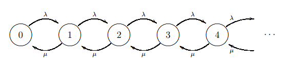
The numbers; 0,1,2,3,4,…….in the circles represent the states. The upward and downward rates are µ and λ. One observes that the transition rate between the states presented in the M/M/1 transition diagram is consistent with the rate of M/M/1’s (280) balanced equations.
The State based Chains of Markov
A Markov chain has two states; include i and j. They communicate if f∃ m, n ≥ 0 and in an instance where pm (i, j ) > 0 and pn (j, i) > 0. Therefore, i can only communicate with j (written i ↔ j ) if one of them reaches the j state from i and vice versa. It is important to note that the relationship between ↔ between I and j should be an equivalence relation. This may be used to separate Markov’s chain and classify them into communication classes. The communication classes refer to sets of disjoints that constitute state space. Each state has a particular communication class whose duty is to communicate with each state of the communication class
(Hannah, 2011).
Conclusion:
According to the study, queuing theory works best for complex system problems. The use of these queues varies depending on the complexity of the system or network environment, and there are several types and uses. The most popular model for several types of queuing procedures is the Markov chains model.
Example 1: You are going to a basketball game and you are entering CIU Arena. To buy tickets, there is just one ticket line. It takes 25 seconds on average to purchase a ticket. Three people arrive on average per minute. Assuming M/M/1 queuing, get the average line length and average waiting time.
Answer:
λ = 3 persons/minute
μ =1/25 persons/seconds = 2.4 persons/minute
p= λ/µ = 3/2.4= 1.25 %
The queue length will explode. The quantity ρ is the fraction of time the server is working.
Consider M/M/1 queue stable with p<1, now ρ >1.
So:
To answer this example we will assume that the ticket purchase takes an average of 15 seconds.
λ = 3 persons/minute
μ =1/15 persons/seconds = 4 persons/minute
p= λ/µ = 3/4= 0.75
Average length of queue
= (0.75)2/(1-0.75)= 2.25 person
Average waiting time in the queue
= 3/ 4 (4 -3) = 0.75 minutes
Example 2: The line to enter the Arena is currently forming. Three turnstiles are in use, each with one ticket taker. An admission ticket taker will process your ticket and provide entry in around three seconds on average. Forty people arrive per minute on average. Assuming M/M/N queuing, get the average queue length and average waiting time.
Answer:
N = 3
Departure rate µ = 3 seconds/person or 20 person/minute
Arrival rate λ = 40 person/minute
p = 40/20 = 2
p/N = 2/3 = 0.667 < 1 so we can use the other equation
p0 = 1/(20 / 0! + 21 / 1! + 22 / 2! + 23 / 3! ( 1 – 2/3)) = 0.1111
Q-bar = (0.1111)(24)/(3! * 3) * (1/(1 – 2/3)2) = 0.88 person
T-bar = (2 + 0.88) / 40 = 0.072 minutes = 4.32 seconds
W-bar = 0.072 – 1/20 = 0.022 minutes = 1.32 seconds
References:
Allen, A. O. (1990). Probability, statistics, and queueing theory. Gulf Professional Publishing.
Allen, A. O. (1992). Probability, statistics, and queueing theory with Computer Science Applications. Gulf Professional Publishing.
Bolch, G., Greiner, S., De Meer, H., & Trivedi, K. S. (2006). Queueing networks and Markov chains: modeling and performance evaluation with computer science applications. John Wiley & Sons.
Constantin, H. (2011). Markov chains and queueing theory. Simulating queuing systems: A test of parameter change, 1-13.
Dattatreya, G. R. (2008). Performance analysis of queuing and computer networks. Chapman and Hall/CRC.
Duffield, N. G. (1994). Exponential bounds for queues with Markovian arrivals. Queueing Systems, 17, 413-430.
Filipowicz, B., & Kwiecień, J. (2008). Queueing systems and networks. Models and applications. Bulletin of the polish academy of sciences technical sciences, 56(4), 379-390.
Gelenbe, E. (1991). Product-form queueing networks with negative and positive customers. Journal of applied probability, 28(3), 656-663.
Gelenbe, E., Glynn, P., & Sigman, K. (1991). Queues with negative arrivals. Journal of applied probability, 28(1), 245-250.
Robertazzi, T. G. (2000). Computer networks and systems: queueing theory and performance evaluation. Springer Science & Business Media.
Trivedi, K. S. (2008). Probability & statistics with reliability, queuing and computer science applications. John Wiley & Sons.
Trivedi, K., 2002. Probability and Statistics with Reliability, Queuing, and Computer Science Applications, 2-nd edition. Wiley & Son, New York.
Van Dijk, N. M. (1993). Queueing Networks and Product Forms: A Systems Approach. John Wiley.
Zukerman, M. (2013). Introduction to queueing theory and stochastic teletraffic models. arXiv preprint arXiv:1307.2968.