

Ali Najah nori1 Walid fahs2
Faculty of Engineering, Computer Communication, Islamic University, Beirut, Lebanon
Email: Neamnbz.85@gmail.com
2 Faculty of Engineering, Computer Communication, Islamic University, Beirut, Lebanon
Email: Walid.fahs@iul.edu.lb
HNSJ, 2023, 4(9); https://doi.org/10.53796/hnsj4913
Published at 01/09/2023 Accepted at 19/08/2023
Abstract
Key Words: Machine learning, model analysis, genetic response, Classification, KNR, Deep learning
Introduction
Seismic waves are vibrations that travel through the Earth as a result of sudden movements within the Earth’s crust, such as earthquakes, volcanic eruptions, landslides, and explosions. These waves can be detected and measured using seismometers.
There are two main types of seismic waves shown in figure 1 body waves and surface waves. Body waves can travel through the Earth’s interior, while surface waves are limited to the Earth’s surface. Body waves are further divided into two types: P-waves (primary waves) and S-waves (secondary waves).
P-waves are the fastest seismic waves and travel through solid and liquid materials. S-waves, on the other hand, can only travel through solid materials and are slower than P-waves.
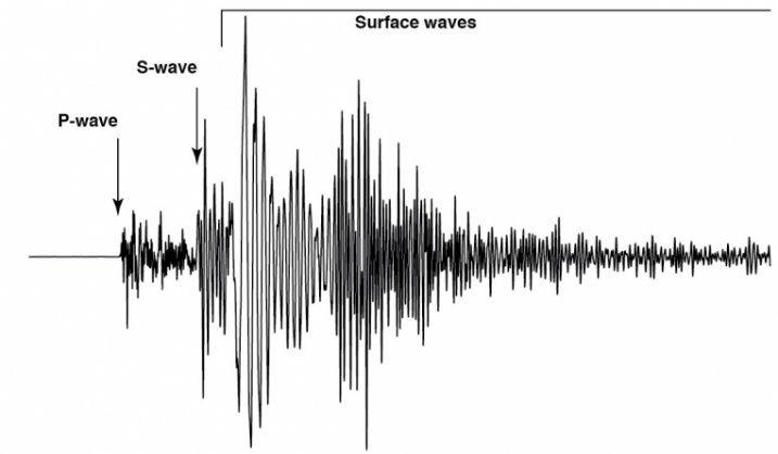
Figure 1 Types of seismic waves
Surface waves, on the other hand, are slower than body waves but can cause more damage at the Earth’s surface. These waves are further divided into two types: Rayleigh waves and Love waves. Rayleigh waves move in a rolling motion, while Love waves move side-to-side. Both types of surface waves are responsible for the shaking and damage that occur during earthquakes [1].
Seismic simulation is a fundamental tool in the field of geophysics used for measuring ground movements, particularly for predicting potential earthquakes. In the oil and gas industry, seismic simulations are used to understand the seismic response of hydrocarbon reservoirs. Geophysical surveys also use seismic simulations to obtain snapshots of the Earth’s interior dynamics and to illuminate its interior through various survey designs. Seismic simulations are crucial in seismic reflection, which aims to estimate the unknown elastic properties of a medium due to its responsiveness .
There are different methods for simulating earthquakes, including finite difference (FD) and spectral element methods [2]. These methods can capture the full range of relevant physics, including the effects of fluid-solid interfaces, intrinsic attenuation, and anisotropy. Both methods estimate the fundamental wave equation to solve for the full seismic wave field propagation [3].
In recent years, various machine learning algorithms have been used to predict seismic waves near oil fields using different features such as frequency, amplitude, and temporal sequence of seismic waves and estimating their strength [4]. This thesis proposes a new method for simulating seismic waves near oil fields using the deep learning algorithm LSTM, comparing its performance with a feature extraction method based on regression to capture the temporal and spectral features of seismic waves using the K-Nearest Neighbors (KNN) regression algorithm on the extracted feature set for predicting the amplitude and frequency characteristics of seismic waves. This is faster and more advanced than traditional iterative numerical methods for full-wave field modeling.
The research enhances predictive accuracy through the utilization of modern techniques, including deep learning algorithms like LSTM, and feature extraction through regression methods such as KNN. These techniques not only surpass traditional numerical methods but also provide insights into seismic activity near oil fields and mining sites. The contributions of this study encompass proposing a novel prediction method, evaluating it against established techniques, highlighting the strengths and limitations of deep learning, and showcasing the potential of machine learning for proactive safety measures. Ultimately, this work aids in the development of more precise and efficient seismic monitoring methods for mining and oil exploration contexts.
This research begins with an introductory overview of fundamental concepts and outlines the content of the subsequent four sections. Section 2, “Literature Review,” delves into relevant studies, methodological approaches, and associated strengths and limitations. In Section 3, “Materials and Methodology,” the proposed system is introduced, presenting the core theoretical foundations, detailing method explanations, and discussing their practical implementation. Section 4, “Results and Discussion,” presents the outcomes of the proposed system, encompassing evaluation methodologies and implementation results. Finally, Section 5, “Conclusions and Future Work,” provides comprehensive conclusions derived from the study and outlines pathways for future research endeavors.
Related Work
These studies cover a range of topics and methodologies related to using machine learning and deep learning techniques for seismic analysis, prediction, and characterization. The studies explore different aspects of seismic data processing, feature extraction, and prediction accuracy. Here’s a brief overview of the key findings and methodologies from each study:
1. Zhen-dong Zhang et al [7]: Developed a deep learning aided elastic full-waveform inversion strategy to extract subsurface facies’ distribution and convert it into reservoir-related parameters using neural networks.
2. [8]: Introduced a deep learning technique using convolutional neural networks (CNN) and support vector machines (SVM) for forecasting hydrocarbon reserves, employing multi-component seismic attributes and clustering techniques.
3. [9]: Proposed a Convolutional Neural Network (CNN) approach for determining Time Delay of Arrival (TDOA) and source location of micro-seismic occurrences in underground mines using cross wavelet transform power and phase spectra.
4. [10]: Utilized Support Vector Regression (SVR) with a focus on porosity and water saturation to extract seismic characteristics and forecast porosity in small data situations.
5. Amin Gholami et al [11]: Presented a mixed model using machine learning to establish articulated seismic characteristics, involving optimized neural networks, support vector regression, and fuzzy logic for improved predictive validity.
6. Léonard Seydoux et al [12]: Created an unsupervised machine learning framework combining deep scattering networks and Gaussian mixture models for identifying seismic signals in continuous seismic data, enabling better prediction of seismic activity.
7. Zachary E. Ross et al [13]: Trained a convolutional neural network to recognize seismic body wave phases, improving phase identification in earthquake monitoring and cataloging.
8. Bertrand Rouet-Leduc et al [14]: Used continuous seismic signals to estimate fault friction, linking seismic signal properties with shear stress and frictional condition using machine learning.
9. Wei Liu et al [15]: Forecasted oil output using an ensemble decomposition method combined with LSTM, ANN, and SVM, demonstrating the superiority of LSTM in predicting oil production.
10. [16]: Documented laboratory earthquakes and showed that slow and fast slip modes are preceded by partial failure events, which can be predicted by training machine learning algorithms on acoustic emissions.
11. Anifowose et al [17]: Explored the use of artificial neural networks, functional networks, support vector machines, and decision trees for determining reservoir porosity and predicting permeability from seismic data.
These studies collectively highlight the potential of machine learning and deep learning techniques in seismic monitoring, including applications in hydrocarbon exploration, earthquake prediction, fault friction estimation, and reservoir characterization. Each study contributes to advancing our understanding and capabilities in the field of seismic monitoring predictions.
The Framework Architecture
The proposed method for Prediction of seismic waves near oil reservoirs using deep learning executed with four main stages, the stages are explained as follows:
-
- Preprocessing stage:
Cleaning and preprocessing the previously collected data is performed to ensure accuracy and remove any missing or irrelevant information. After reading the seismic wave readings dataset, the data is cleaned and organized. This stage is referred to as preprocessing and is the first step in this process, involving filling in any missing values using various strategies. For instance, calculating the standard deviation of the feature set and filling the missing values with this value..
- Missing value
Missing values can lead to a loss of valuable information and arise when certain observations lack recorded values. During the preprocessing phase, mean imputation is employed to approximate missing values in the seismic wave data. This method involves replacing missing values with the mean value of the other entries within the same column. For this project, a modification will be made to the mean imputation approach, utilizing the mean value of comparable days rather than considering all blood samples collectively.
- Normalization
An additional preprocessing procedure involves min-max normalization, often referred to as feature scaling. This method entails applying a linear transformation to the data, effectively rescaling it within a range of (0, 1) [18]. The normalization process is carried out in accordance with equation (1):
(1)
Where represent normalized .
-
- Feature selection stage
In machine learning, correlation can be used in feature selection to identify the features that have the strongest relationship with the target variable. By identifying the features that are most correlated with the target variable, we can select the most informative features and use them in our model. Correlation can also be used to identify and remove features that are highly correlated with other features, as these features may not add much additional information to the model. One common method for feature selection is to use a correlation matrix to identify the features with the highest correlation with the target variable and use those features in the model.
Regarding feature selection, if two features are found to be highly correlated based on the correlation matrix, only one of them will be retained. Additionally, any features that exhibit a correlation of ‘thres=0.9’ or higher with another feature will also be removed. The feature selection process shown in figure 2.
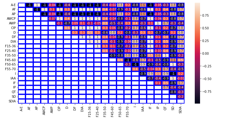
Figure 2: the feature selection pre-processing method.
In figure 2 After applying correlation analysis, 11 highly correlated features were removed from the dataset, namely: [‘AP’, ‘AWCP’, ‘CIP’, ‘DF’, ‘DIA’, ‘F15-36’, ‘F25-40’, ‘IF’, ‘IP’, ‘QT’, ‘SD’]. The remaining dataset was reduced to 11 features, namely [‘A-E’,’AF’,’AWP’,’D’,’F35-50’,’F45-60’,’F50-65’,’F55-70 I’,’IAA’,’SDIA’].
In the next step, we Converting a time series data to a supervised learning dataset involves using the previous time steps as input features and the current time step as the output feature. In other words, the model uses historical data to predict the current value.
The function `series_to_supervised` is used to create a supervised learning dataset from a time series data. It takes in parameters such as the data, the number of lag observations as input, the number of future observations to predict as output, and a boolean flag to indicate whether or not to drop rows with NaN values.
In the current application, the ground wave data is sampled daily, so the input is the previous day, and the output is the current day. This means that the function will sample {t – n, t – n – 1, …, t – 1} as input features and {t, t+1, …, t+n} as output features.
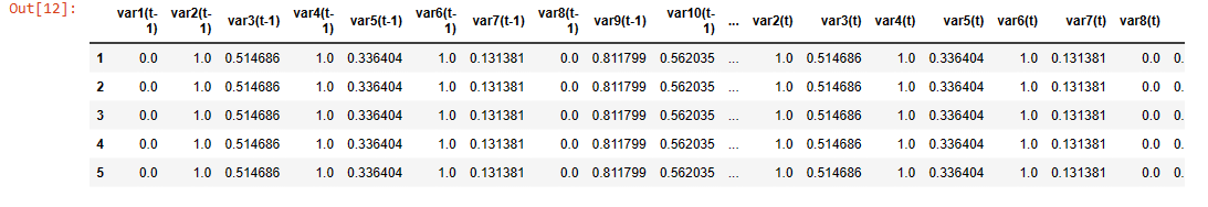
Figure 3: The supervised learning dataset.
The resulting dataset will be used to train a machine learning model to predict the ground wave data for future time steps based on historical data. Figures 3 and 4 converting a time series data to a supervised learning dataset.
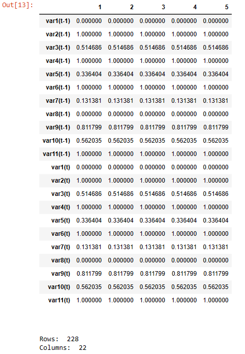
Figure 4 : The shape of supervised learning dataset.
It is necessary to eliminate unimportant features and retain only the important ones. The following method used for this purpose:
-
- Machine learning stage
Machine learning algorithms have the capacity to address challenges spanning various domains and streamline the management of data.
- K-Nearest Neighbors Regression (KNR)
The K-Nearest Neighbors Regression (KNR) algorithm makes use of the concept of feature similarity’ in order to predict the values of new data points. In other words, a new point is assigned a value based on how closely it resembles the existing points in the training set [19].
-
- Deep learning
Deep learning is a branch of machine learning that uses artificial neural networks. These networks (as depicted in figure 5), consist of layers of interconnected nodes called neurons, which process and learn from input data. In a deep neural network, there’s an input layer followed by hidden layers, each connected to the previous one. Neurons receive input from the previous layer and pass output to the next layer, culminating in the final output layer. Through nonlinear transformations, these layers transform input data, enabling the network to learn complex patterns and representations [20].
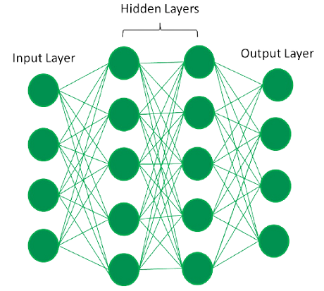
Figure 5: The fully connected deep neural network
In neural networks, connections between layers have weights. Inputs are multiplied by weights and summed in units. This sum goes through activation functions like sigmoid, tanh, or ReLU(as shown in figure 6 ). These functions reshape output. Sigmoid curves between 0 and 1 but has issues like vanishing gradients. Tanh ranges from -1 to 1 and handles vanishing gradients better. ReLU is simple and efficient, addressing vanishing gradient problems, but can lead to dead neurons. These functions are picked for favorable derivatives. Output from activation feeds the next layer. The final output layer solves the problem [21].
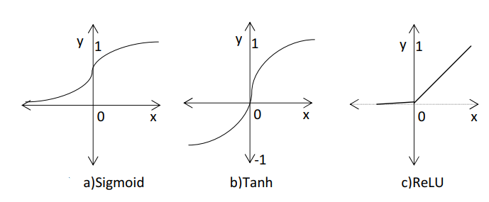
Figure 6: The activation functions [18]
- LONG-SHORT-TERM MEMORY (LSTM)
The Long Short-Term Memory (LSTM) model is a type of recurrent neural network designed to address learning long-term dependencies and gradient problems in sequential data. It employs memory cells and three gates: input, forget, and output. The input gate adds new information, the forget gate discards irrelevant data, and the output gate controls what’s exposed. LSTMs excel in tasks like language processing and time series analysis. Variations with different gating mechanisms, peephole connections, and activation functions have been explored for better performance. Unfortunately, I can’t view external figures, so I can’t comment on “figure 7.”[22].
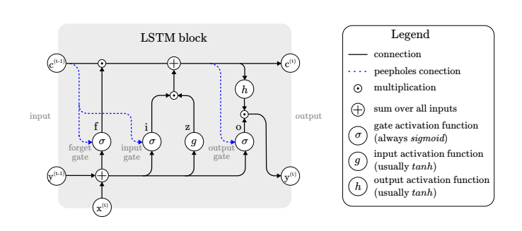
Figure 7: Long Short-Term Memory (LSTM) model [22]
3.4 Methodology
The suggested framework, illustrated in “Figure 8,” encompasses four key stages. The initial stage involves pre-processing, encompassing both the handling of missing values and normalization procedures. Following this, the second stage involves the utilization of feature selection methods to identify a subset of pertinent features.
Subsequently, the dataset is subjected to classification using both Machine Learning (ML) and Deep Learning (DL) models in the third stage. Finally, the performance assessment of the proposed system is carried out using the accuracy metric.
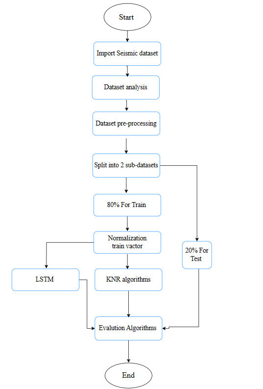
Figure 8: Block diagram of main stages for proposed model
IV. RESULTS AND DISCUSSION
- Dataset
The seismic wave prediction task uses a dataset with 230 rows and 22 features from real seismic monitoring locations, represented in a CSV file. The dataset’s relationships are explored using a heatmap, as depicted in Figure 9. This visualization helps identify correlations between variables. Dark colors signify strong positive correlations, while lighter colors indicate weaker or negative correlations. The analysis aims to find patterns and influential variables for predicting seismic waves accurately. Other techniques include descriptive statistics for understanding data tendencies, correlation analysis for measuring relationships, PCA for dimensionality reduction, and machine learning for predictive model development. These methods collectively provide insights into the dataset and support effective seismic wave prediction modeling.
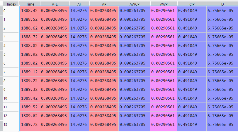
Figure 9: A sample of the original gene data in CSV file
- Pre-processing
Considering the dataset employed in this investigation, two preliminary preprocessing measures were deemed necessary for facilitating the model implementation. The initial measure revolved around tackling the presence of missing values within the unprocessed data.
Within the dataset, certain attributes were devoid of values, thus designated as NaN (Not a Number). To rectify this, a solution was devised by computing the mean value of the associated column, one that contained values for the identical attribute. This computation was executed employing equation (4), effectively approximating and inferring the absent values for all residual samples..
(4)
Let X denote the data value, and N signify the count of data values within a specific column. Another crucial step entailed in the preprocessing entailed Min-Max normalization, which was enacted in accordance with equation (1).
Subsequent to the execution of the aforementioned processes, the result manifested as a dataset exhibiting an identical count of features and samples in comparison to the initial dataset. Nonetheless, the distinction emerged in terms of the actual data values, given that the absent values had been appropriately addressed and rectified.
Furthermore, an essential aspect of this transformation lay in adjusting the data to satisfy the requisite range prerequisites.
- Machine and Deep Learning Models
The proposed system focuses on predicting seismic waves using regression-based machine learning techniques, particularly the LSTM (Long Short-Term Memory) algorithm. LSTM excels in capturing complex temporal patterns and handling long-term dependencies in time-series data. The system also emphasizes the application of the KNR (K-Nearest Neighbor Regression) algorithm.
The training process involves splitting the preprocessed seismic wave dataset into training and validation sets. The LSTM model is initialized with random weights and biases, and during training epochs, forward propagation makes predictions. A suitable loss function (MAE or RMSE) quantifies prediction errors. Backpropagation calculates gradients for parameter updates via optimization algorithms like SGD or Adam. Hyperparameters are fine-tuned for optimal performance, and training continues until convergence or a set number of epochs. The trained model is saved for predicting seismic waves near oil fields, contributing to early detection and prevention of potential damage.
The testing phase uses a distinct test dataset with the same distribution as the training data. The trained model is evaluated on this test set, assessing its ability to generalize to new and unseen data. This evaluation provides valuable insights into the model’s accuracy and effectiveness in predicting seismic waves in real-world scenarios. The separation of the test set ensures unbiased evaluation and ensures the system’s reliability for early detection and prevention in oil fields. The training curve for LSTM shown in figure 10 and 11.
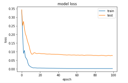
Figure 10: The loss curve of LSTM
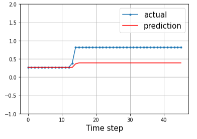
Figure 11: The predict curve of LSTM
Figures 4.5 – 4.7 illustrate the LSTM network training and testing process, which resulted in very low error rates. This indicates the accuracy of the achieved results.
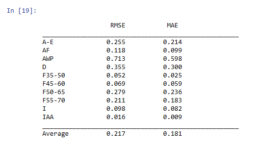
Figure 12: The predict curve of LSTM
Figure 12 provides evaluation metrics for the LSTM model on different performance measures, namely Root Mean Squared Error (RMSE) and Mean Absolute Error (MAE) for different target variables. The target variables are abbreviated in the first column. RMSE values range from 0.016 to 0.713, while MAE values range from 0.009 to 0.598.
The average values of RMSE and MAE across all target variables are 0.217 and 0.181, respectively. These values indicate that the LSTM model performs well in predicting seismic waves near oil fields.
The K-Nearest Neighbors Regression (KNR) algorithm predicts values for new data based on similarity to existing training points. Accuracy is evaluated using metrics like mean absolute error (MAE) and root mean squared error (RMSE).
In training and testing, the dataset is split. Training teaches the model relationships by measuring distances to nearest neighbors, with a tunable neighbor count (k). Testing assesses model performance by comparing predictions to actual values. Metrics like MAE and RMSE measure error magnitude, with lower values indicating better performance (see Figure 13).

Figure 13 the training and testing step OF KNR.
Figure 13 shows that the average RMSE and MAE values for the KNR model are 0.485 and 0.538, respectively. This means that the KNR model has a relatively higher error compared to the LSTM model in predicting seismic waves near oil fields.
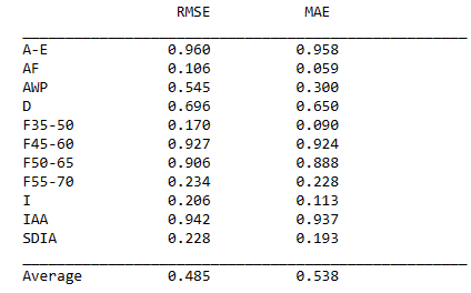
Figure 14: the RMSE and MAE for KNR
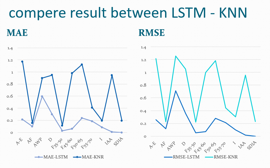
Figure 15: compere result between LSTM – KNR.
Figure 15 presents the comparison of results between the LSTM and KNN algorithms. As this visual representation highlights the differences in performance between the two algorithms, we note that in terms of prediction accuracy, the LSTM algorithm is superior.
- CONCLUSION
In this study, we trained and evaluated two distinct models, LSTM and KNR, for predicting various air quality parameters. The LSTM model consistently demonstrated superior performance compared to the KNR model, evident through lower RMSE and MAE values across most of the predicted parameters. The LSTM model exhibited strong predictive capabilities with RMSE values spanning from 0.026 to 0.958 and MAE values ranging from 0.014 to 0.958. While the KNR model displayed satisfactory performance for certain parameters, its performance varied, resulting in RMSE values ranging from 0.106 to 0.942 and MAE values ranging from 0.059 to 0.937 for different predicted parameters.
References
[1] Michigan Technological University. (n.d.). Seismology Study. Retrieved [Access Date], from https://www.mtu.edu/geo/community/seismology/learn/seismology-study/.
[2] Y. Cui, K. B. Olsen, T. H. Jordan, K. Lee, J. Zhou, P. Small, D. Roten, G. Ely, D. K. Panda, A. Chourasia, J. Levesque, S. M. Day, and P. Maechling, “Scalable earthquake simulation on petascale supercomputers,” in 2010 ACM/IEEE International Conference for High Performance Computing, Networking, Storage and Analysis (2010) pp. 1–20.
[3] P. Lubrano-Lavadera, ˚A. Drottning, I. Lecomte, B.D.E. Dando, D. K¨uhn, and V. Oye, “Seismic modelling: 4d capabilities for co2 injection,” Energy Procedia 114, 3432 – 3444 (2017).
[4] G. Schuster, Seismic Inversion (Society of Exploration Geophysicists, 2017).
[5] . Moseley, B., Markham, A., & Nissen-Meyer, T. (2018). Fast approximate simulation of seismic waves with deep learning. arXiv preprint arXiv:1807.06873.
[6] A. Richardson, “Seismic Full-Waveform Inversion Using Deep Learning Tools and Techniques,” ArXiv e-prints (2018).
[7] Zhang, Z., & Alkhalifah, T. (2020). High-resolution reservoir characterization using deep learning aided elastic full-waveform inversion: The North Sea field data example. GEOPHYSICS, 1–47. doi:10.1190/geo2019-0340.1.
[8] FU Chao, LIN NianTian, ZHANG Dong, WEN Bo, WEI QianQian, ZHANG Kai. 2018. Prediction of reservoirs using multi-component seismic data and the deep learning method. Chinese Journal of Geophysics (in Chinese), 61(1): 293-303, doi: 10.6038/cjg2018L0193”.
[9] L.Huangac,JunLic,H.Haobc,X.Lia,” Micro-seismic event detection and location in underground mines by using Convolutional Neural Networks (CNN) and deep learning”,2018, https://doi.org/10.1016/j.tust.2018.07.006 .
[10] S. R. Na’imi, S. R. Shadizadeh, M. A. Riahi, and M. Mirzakhanian, “Estimation of reservoir porosity and water saturation based on seismic attributes using support vector regression approach,” J. Appl. Geophys., vol. 107, pp. 93–101, 2014, doi: 10.1016/j.jappgeo.2014.05.011.
[11] A. Gholami and H. R. Ansari, “Estimation of porosity from seismic attributes using a committee model with bat-inspired optimization algorithm,” J. Pet. Sci. Eng., vol. 152, no. March, pp. 238–249, 2017, doi: 10.1016/j.petrol.2017.03.013.
[12] Seydoux, L., R. Balestriero, P. Poli, M. De Hoop, M. Campillo, and R. Baraniuk (2020) “Clustering earthquake signals and background noises in continuous seismic data with unsupervised deep learning,” Nature communications, 11(1), pp. 1–12.
[13] Ross, Z. E., M.-A. Meier, E. Hauksson, and T. H. Heaton (2018) “Generalized seismic phase detection with deep learning,” Bulletin of the Seismological Society of America, 108(5A), pp. 2894–2901.
[14] Rouet-Leduc, B., C. Hulbert, D. C. Bolton, C. X. Ren, J. Riviere, C. Marone, R. A. Guyer, and P. A. Johnson (2018) “Estimating fault friction from seismic signals in the laboratory,” Geophysical Research Letters, 45(3), pp. 1321–1329.
[15] “Seismic survey.” In Encyclopædia Britannica. Retrieved May 13, 2023, from https://www.britannica.com/science/seismic-survey.
[16] Poursartip, B., Fathi, A., & Tassoulas, J. L. (2020). Large-scale simulation of seismic wave motion: A review. Soil Dynamics and Earthquake Engineering, 129, 105909. https://doi.org/10.1016/j.soildyn.2019.105909.
[17] Galkina, A. and N. Grafeeva (2019) “Machine learning methods for earthquake prediction: A survey,” Proc. SEIM, p. 25.
[18] K. Asim, A. Idris, T. Iqbal, and F. Martínez-Álvarez, “Earthquake prediction model using support vector regressor and hybrid neural networks,” PLOS ONE, vol. 13, 2018..
[19] MIT Sloan School of Management. “Machine Learning, Explained.” Ideas Made to Matter, 28 Feb. 2018, mitsloan.mit.edu/ideas-made-to-matter/machine-learning-explained.
[20] J. Bi, Y. Wang, X. Li, H. Qi, H. Cao, and S. Xu, ‘‘An adaptive weighted KNN positioning method based on omnidirectional fingerprint database and twice affinity propagation clustering,’’ Sensors, vol. 18, no. 8, p. 2502, Aug. 2018.
[20] S. Zhang, X. Li, M. Zong, X. Zhu and R. Wang, “Efficient kNN classification with different numbers of nearest neighbors”, IEEE Trans. Neural Netw. Learn. Syst., vol. 29, no. 5, pp. 1774-1785, May 2018.
[21] Buza K, Nanopoulos A, Nagy G (2015) Nearest neighbor regression in the presence of bad hubs. Knowl Based Syst 86:250–260.
[22] Dubey, S. R., Singh, S. K., & Chaudhuri, B. B. (2022). Activation functions in deep learning: A comprehensive survey and benchmark. Neurocomputing, 496, 96-123. https://doi.org/10.1016/j.neucom.2022.06.111